
Import Library
import numpy as npimport pandas as pdimport seaborn as snsimport matplotlib.pyplot as pltimport warningswarnings.filterwarnings('ignore')
Load data
data = pd.read_csv('INDIAVIX.csv')Domain Analysis
-
Date: The specific day when the stock prices are recorded.
-
Open: The price at which the stock started trading at the beginning of the day.
-
High: The highest price at which the stock traded during the day.
-
Low: The lowest price at which the stock traded during the day.
-
Close: The price at which the stock ended trading at the end of the day.
-
Previous: The closing price of the stock from the previous trading day.
-
Change: The difference between the closing price of the current day and the previous day’s closing price.
-
PerChange: The percentage change in the stock’s closing price compared to the previous day’s closing price.
Basic Check
data.head()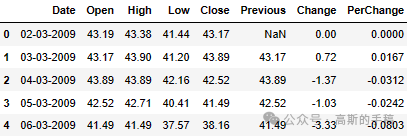
data.tail()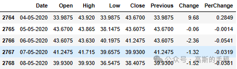
data.columnsIndex(['Date', 'Open', 'High', 'Low', 'Close', 'Previous', 'Change',
'PerChange'],
dtype=’object’)
data.dtypesDate object Open float64 High float64 Low float64 Close float64 Previous float64 Change float64 PerChange float64 dtype: object
data.info()<class 'pandas.core.frame.DataFrame'>RangeIndex: 2769 entries, 0 to 2768Data columns (total 8 columns): # Column Non-Null Count Dtype --- ------ -------------- ----- 0 Date 2769 non-null object 1 Open 2769 non-null float64 2 High 2769 non-null float64 3 Low 2769 non-null float64 4 Close 2769 non-null float64 5 Previous 2768 non-null float64 6 Change 2769 non-null float64 7 PerChange 2769 non-null float64dtypes: float64(7), object(1)
memory usage: 173.2+ KB
data.describe()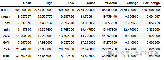
data.Change.value_counts()0.00 29
-0.05 24
-0.06 23
-0.16 22
-0.37 22
..
3.65 1
1.87 1
1.43 1
2.74 1
-2.36 1
Name: Change, Length: 532, dtype: int64
Data Preprocessing
data.corr()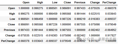
# Checking mean median and modeprint(data.mean())print(data.median())print(data.mode())
Open         19.637037
High         20.550775
Low          18.297726
Close        19.765841
Previous     19.759440
Change       -0.000968
PerChange     0.001347
dtype: float64
Open         17.24750
High         17.99000
Low          16.05750
Close        17.27500
Previous     17.27375
Change       -0.04000
PerChange    -0.00220
dtype: float64
            Date   Open   High    Low  Close  Previous  Change  PerChange
0     01-01-2013  16.82  16.91  16.17  14.25     14.25     0.0        0.0
1     01-01-2014    NaN  21.22    NaN  14.51     14.51     NaN        NaN
2     01-01-2015    NaN    NaN    NaN  15.55     15.55     NaN        NaN
3     01-01-2016    NaN    NaN    NaN  16.16     16.16     NaN        NaN
4     01-01-2018    NaN    NaN    NaN  16.36     16.36     NaN        NaN
...          ...    ...    ...    ...    ...       ...     ...        ...
2764  31-12-2013    NaN    NaN    NaN    NaN       NaN     NaN        NaN
2765  31-12-2014    NaN    NaN    NaN    NaN       NaN     NaN        NaN
2766  31-12-2015    NaN    NaN    NaN    NaN       NaN     NaN        NaN
2767  31-12-2018    NaN    NaN    NaN    NaN       NaN     NaN        NaN
2768  31-12-2019    NaN    NaN    NaN    NaN       NaN     NaN        NaN

[2769 rows x 8 columns]
# Converting 'Date' is the column containing date objects# Convert 'Date' column to datetime with the correct formatdata["Date"] = pd.to_datetime(data["Date"], format='%d-%m-%Y')# Extract day, month, and year into separate columnsdata['Day'] = data['Date'].dt.daydata['Month'] = data['Date'].dt.monthdata['Year'] = data['Date'].dt.year
data = data.dropna(subset=['Previous'])data.isnull().sum()Date 0 Open 0 High 0 Low 0 Close 0 Previous 0 Change 0 PerChange 0 Day 0 Month 0 Year 0 dtype: int64
data.dtypesDate datetime64[ns] Open float64 High float64 Low float64 Close float64 Previous float64 Change float64 PerChange float64 Day int64 Month int64 Year int64 dtype: object
Exploratory Data Analysis
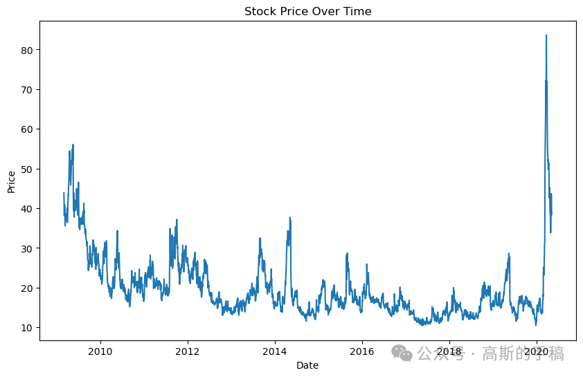
#Line Plotplt.figure(figsize=(10, 6))plt.plot(data['Date'], data['Close'])plt.title('Stock Price Over Time')plt.xlabel('Date')plt.ylabel('Price')plt.show()
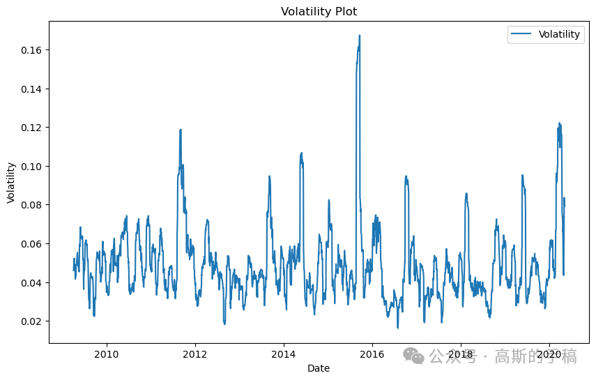
plt.figure(figsize=(10, 6))plt.plot(data['Date'], data['Close'].pct_change().rolling(window=20).std(), label='Volatility')plt.title('Volatility Plot')plt.xlabel('Date')plt.ylabel('Volatility')plt.legend()plt.show()
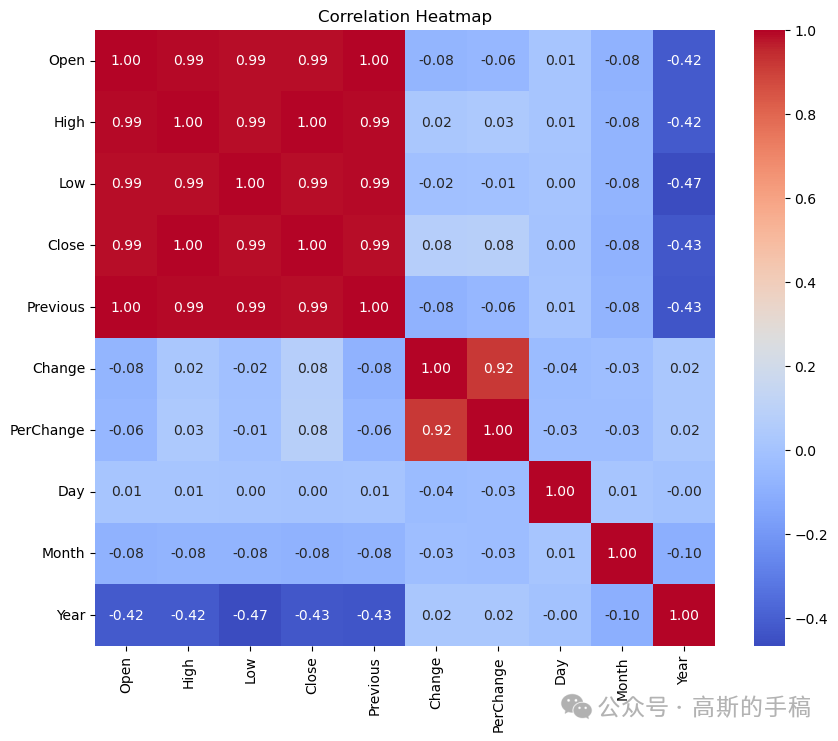
# The heatMap plotcorr_matrix = data.corr()plt.figure(figsize=(10, 8))sns.heatmap(corr_matrix, annot=True, cmap='coolwarm', fmt=".2f")plt.title('Correlation Heatmap')plt.show()
sns.displot(x=data['Change'])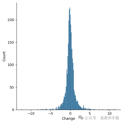
from autoviz.AutoViz_Class import AutoViz_ClassAV=AutoViz_Class()data=AV.AutoViz(filename="INDIAVIX.csv",verbose=2,chart_format='html')
Feture Engineering
sns.pairplot(data)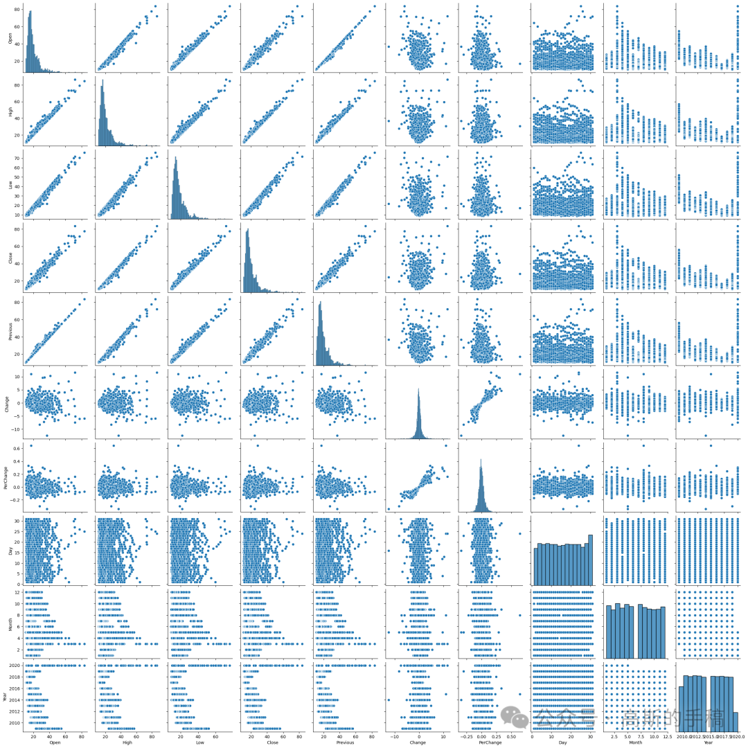
data.corr()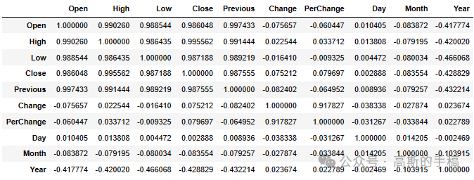
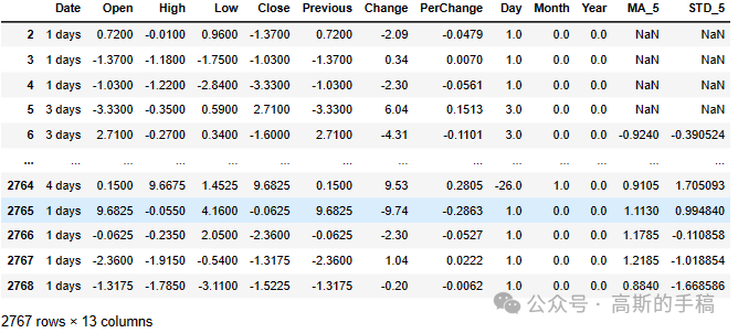
# Here I'm creating seprate colomns for MA_5 and STD_5 who's based on close of mean and standered daviationdata['MA_5'] = data['Close'].rolling(window=5).mean()data['STD_5'] = data['Close'].rolling(window=5).std()
Stationarity
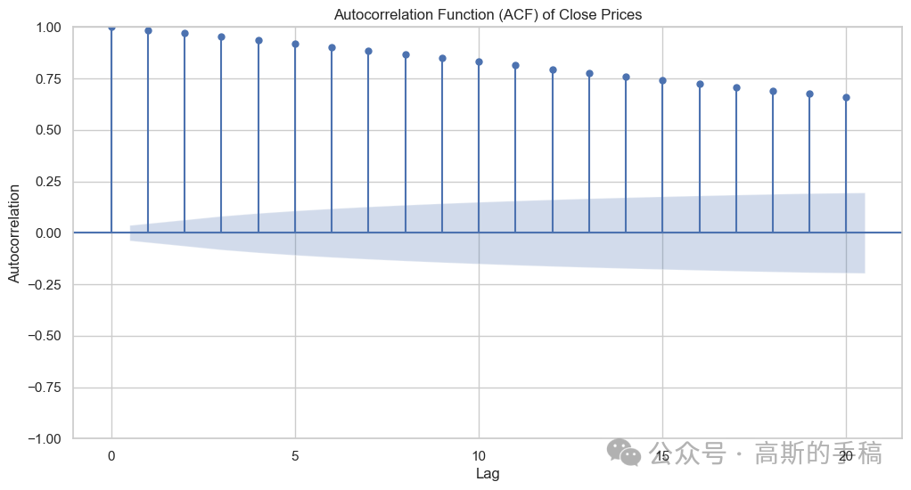
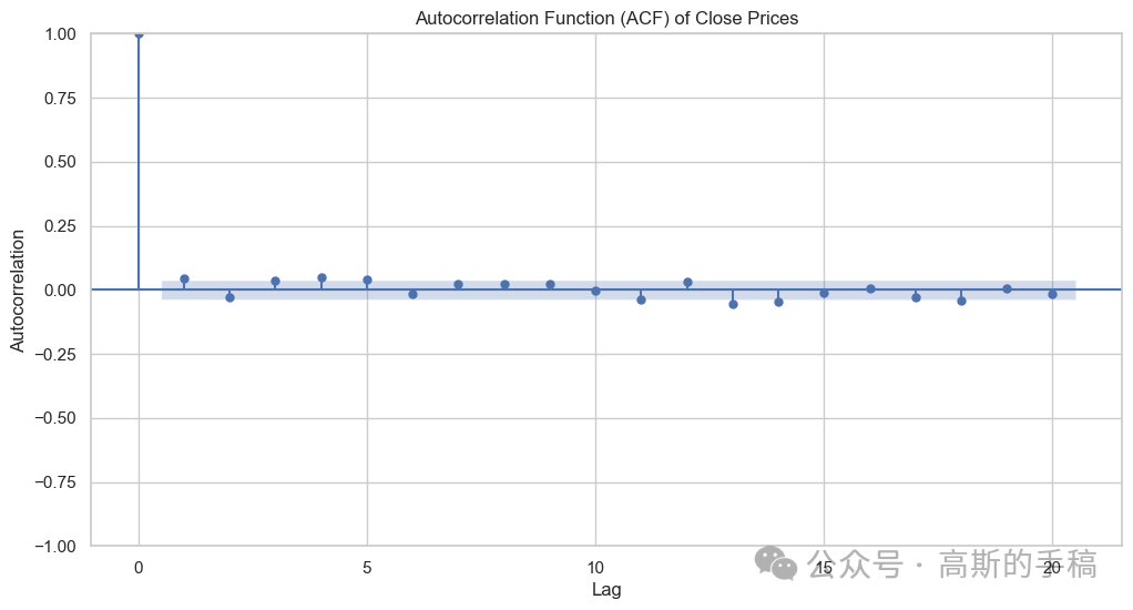
## Plotting the autocorrelation functionfrom statsmodels.graphics.tsaplots import plot_acf# Set up the figure and axes using seaborn styleplt.figure(figsize=(12, 6))sns.set(style='whitegrid')# Plot the ACF using plot_acf from statsmodelsplot_acf(data['Close'], lags=20, alpha=0.05, ax=plt.gca())plt.title('Autocorrelation Function (ACF) of Close Prices')plt.xlabel('Lag')plt.ylabel('Autocorrelation')plt.show()
from statsmodels.tsa.stattools import adfuller# Assuming 'data' is your DataFrame with stock data, and 'Close' is the column of interestdftest = adfuller(data['Close'], autolag='AIC')# Extract and print resultsprint("Results of Augmented Dickey-Fuller Test:")print("ADF Statistic: %f" % dftest[0])print("P-value: %f" % dftest[1])print("Number of Lags Used: %d" % dftest[2])print("Number of Observations Used: %d" % dftest[3])print("Critical Values:")for key, val in dftest[4].items():print("\t%s: %.3f" % (key, val))# Interpret the resultsif dftest[1] <= 0.05:print("Conclusion: Reject the null hypothesis.")print("The data is stationary.")else:print("Conclusion: Fail to reject the null hypothesis.")print("The data is non-stationary.")
Results of Augmented Dickey-Fuller Test:ADF Statistic: -3.951116P-value: 0.001689Number of Lags Used: 23Number of Observations Used: 2744Critical Values: 1%: -3.433 5%: -2.863 10%: -2.567Conclusion: Reject the null hypothesis.
The data is stationary.
data1=data.diff(periods=1)data1=data1.iloc[1:] #null value discardedata1
## Plotting the autocorrelation function # Set up the figure and axes using seaborn styleplt.figure(figsize=(12, 6))sns.set(style='whitegrid')# Plot the ACF using plot_acf from statsmodelsplot_acf(data1['Close'], lags=20, alpha=0.05, ax=plt.gca()) plt.title('Autocorrelation Function (ACF) of Close Prices')plt.xlabel('Lag')plt.ylabel('Autocorrelation') plt.show()
data2=data1.diff(periods=1) # differencing applied to data1data2=data2.iloc[1:] # integrated to the order of 2## Plotting the autocorrelation function# Set up the figure and axes using seaborn styleplt.figure(figsize=(12, 6))sns.set(style='whitegrid')# Plot the ACF using plot_acf from statsmodelsplot_acf(data1['Close'], lags=20, alpha=0.05, ax=plt.gca())plt.title('Autocorrelation Function (ACF) of Close Prices')plt.xlabel('Lag')plt.ylabel('Autocorrelation')plt.show()
Model Building
# Select the Close price columnclose_data = data['Close']# Split the data into training and testing setstrain_size = int(len(data) * 0.8)train, test = close_data[:train_size], close_data[train_size:]
train.info()#info about datatype and null value
<class 'pandas.core.series.Series'>Int64Index: 2214 entries, 1 to 2214Series name: CloseNon-Null Count Dtype -------------- ----- 2214 non-null float64dtypes: float64(1)memory usage: 34.6 KB
Autoregressive model
## Applying autoregressive model#from statsmodels.tsa.ar_model import AR##from statsmodels.tsa.ar_model import AutoRegfrom statsmodels.tsa.ar_model import ar_select_order, AutoRegimport warningswarnings.filterwarnings('ignore')
# Use ar_select_order to find the best lagsmod = ar_select_order(close_data, maxlag=15, glob=True)best_lags = mod.ar_lagsprint("Best lags:", best_lags)
# fitting Modelar_model = AutoReg(train, lags=best_lags)ar_model_fit = ar_model.fit()# Summary of the modelprint(ar_model_fit.summary())
AutoReg Model Results ==============================================================================Dep. Variable: Close No. Observations: 2214Model: Restr. AutoReg(10) Log Likelihood -3488.602Method: Conditional MLE S.D. of innovations 1.178Date: Fri, 14 Jun 2024 AIC 6985.204Time: 03:50:55 BIC 7007.996Sample: 10 HQIC 6993.532 2214 ============================================================================== coef std err z P>|z| [0.025 0.975]------------------------------------------------------------------------------const 0.2556 0.075 3.412 0.001 0.109 0.402Close.L1 0.9699 0.008 116.043 0.000 0.954 0.986Close.L10 0.0167 0.008 2.032 0.042 0.001 0.033 Roots ============================================================================== Real Imaginary Modulus Frequency------------------------------------------------------------------------------AR.1 1.0117 -0.0000j 1.0117 -0.0000AR.2 1.3097 -0.5968j 1.4393 -0.0680AR.3 1.3097 +0.5968j 1.4393 0.0680AR.4 0.6722 -1.4050j 1.5575 -0.1790AR.5 0.6722 +1.4050j 1.5575 0.1790AR.6 -0.3682 -1.5742j 1.6167 -0.2866AR.7 -0.3682 +1.5742j 1.6167 0.2866AR.8 -1.6566 -0.0000j 1.6566 -0.5000AR.9 -1.2913 -1.0226j 1.6471 -0.3934AR.10 -1.2913 +1.0226j 1.6471 0.3934
# Forecaststart = len(train)end = len(train) + len(test) - 1ar_predictions = ar_model_fit.predict(start=start, end=end, dynamic=False)# Ensure no NaN values in predictionsar_predictions = ar_predictions.dropna()test = test[:len(ar_predictions)]
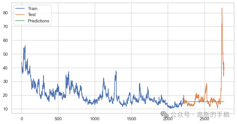
# Evaluate the modelfrom sklearn.metrics import mean_squared_errorrmse = mean_squared_error(test, ar_predictions, squared=False)print(f'RMSE: {rmse}')# Plotplt.figure(figsize=(10, 5))plt.plot(train.index, train, label='Train')plt.plot(test.index, test, label='Test')plt.plot(ar_predictions.index, ar_predictions, label='Predictions')plt.legend()plt.show()

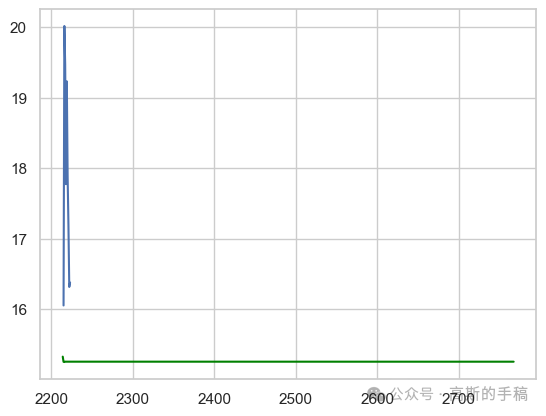
# Plotplt.plot(test)plt.plot(ar_predictions,color='green') #graph of test vs prediction
ARIMA Model
## importing the libraryfrom statsmodels.tsa.arima.model import ARIMA
# Determine the optimal order for ARIMA model (using the best AR lags for p, and setting d=1 and q=0)p = len(best_lags)d = 1q = 0# Split the data into training and testing setstrain_size = int(len(close_data) * 0.8)train, test = close_data[:train_size], close_data[train_size:]# Fit the ARIMA modelarima_model= ARIMA(train, order=(p, d, q))arima_model_fit = arima_model.fit()# Summary of the modelprint(arima_model_fit.summary())
SARIMAX Results ==============================================================================Dep. Variable: Close No. Observations: 2214Model: ARIMA(2, 1, 0) Log Likelihood -3519.079Date: Fri, 14 Jun 2024 AIC 7044.158Time: 03:51:13 BIC 7061.265Sample: 0 HQIC 7050.407 - 2214 Covariance Type: opg ============================================================================== coef std err z P>|z| [0.025 0.975]------------------------------------------------------------------------------ar.L1 -0.0322 0.011 -2.882 0.004 -0.054 -0.010ar.L2 -0.0623 0.014 -4.548 0.000 -0.089 -0.035sigma2 1.4084 0.016 86.859 0.000 1.377 1.440===================================================================================Ljung-Box (L1) (Q): 0.02 Jarque-Bera (JB): 14819.01Prob(Q): 0.90 Prob(JB): 0.00Heteroskedasticity (H): 0.33 Skew: -0.04Prob(H) (two-sided): 0.00 Kurtosis: 15.68==================================================================================
# Forecaststart = len(train)end = len(train) + len(test) - 1arima_predictions = arima_model_fit.predict(start=start, end=end, dynamic=False)# Ensure no NaN values in predictionsarima_predictions = arima_predictions.dropna()test = test[:len(arima_predictions)]
# Evaluate the modelfrom sklearn.metrics import mean_squared_errorrmse = mean_squared_error(test, arima_predictions, squared=False)print(f'RMSE: {rmse}')# Plotplt.figure(figsize=(10, 5))plt.plot(train.index, train, label='Train')plt.plot(test.index, test, label='Test')plt.plot(arima_predictions.index, arima_predictions, label='Predictions')plt.legend()plt.show()
# Ensure no NaN values in predictionsar_predictions = ar_predictions.dropna()test_ar = test[:len(ar_predictions)]
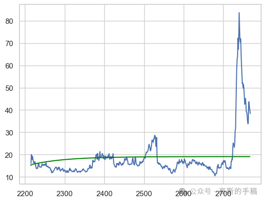
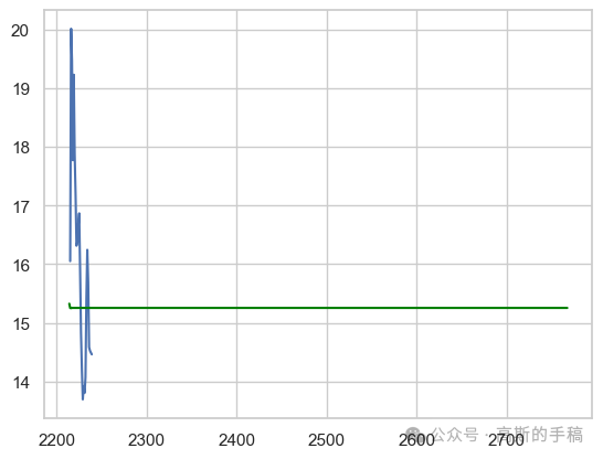
# Comparision of actual vs predicted for 9 valuesplt.plot(test[:9])plt.plot(arima_predictions,color='green')#line plot for prediction
# Comparision of actual vs predicted for 25 valuesplt.plot(test[:25])plt.plot(arima_predictions,color='green') #line plot for prediction
Model Evaluation ARIMA
import numpy as npfrom sklearn.metrics import mean_squared_errorfrom statsmodels.tools.eval_measures import rmse# Define the accuracy metrics functiondef forecast_accuracy(forecast, actual):mse = np.mean((forecast - actual)**2) # Mean Squared Error (MSE)mae = np.mean(np.abs(forecast - actual)) # Mean Absolute Error (MAE)rmse = np.mean((forecast - actual)**2)**.5 # Root Mean Squared Error (RMSE)return {'mse': mse, 'mae': mae, 'rmse': rmse}# Assuming forecast25 and test1 are your forecasted and actual values respectivelyforecast25 = arima_predictionstest1 = test
# Calculate and print accuracy metricsaccuracy_metrics = forecast_accuracy(forecast25, test1)print("Accuracy metrics:", accuracy_metrics)# Calculate and print RMSE using statsmodelsprint("RMSE (statsmodels):", rmse(test1, forecast25))# Calculate and print MSE using sklearnprint("MSE (sklearn):", mean_squared_error(test1, forecast25))
from sklearn.metrics import mean_squared_errorfrom statsmodels.tools.eval_measures import rmse# Calculate root mean squared errorprint(rmse(test1, forecast25))# Calculate mean squared errormean_squared_error(test1, forecast25)
# Ensure no NaN values in predictionsarima_predictions = arima_predictions.dropna()test_arima = test[:len(arima_predictions)]
Conclusion
# Calculate accuracy metrics for AR modelar_accuracy = forecast_accuracy(ar_predictions, test_ar)print("The AR model accuracy metrics:", ar_accuracy)# Calculate accuracy metrics for ARIMA modelarima_accuracy = forecast_accuracy(arima_predictions, test_arima)print("The ARIMA model accuracy metrics:", arima_accuracy)# Additional metrics using sklearn and statsmodelsprint("The AR model RMSE (statsmodels):", rmse(test_ar, ar_predictions))print("The AR model MSE (sklearn):", mean_squared_error(test_ar, ar_predictions))print("The ARIMA model RMSE (statsmodels):", rmse(test_arima, arima_predictions))print("The ARIMA model MSE (sklearn):", mean_squared_error(test_arima, arima_predictions))
The AR model accuracy metrics: {'mse': 102.29256679864773, 'mae': 5.529926168061879, 'rmse': 10.113978781797385}The ARIMA model accuracy metrics: {'mse': 114.96755895589818, 'mae': 4.591014924243197, 'rmse': 10.72229261659549}The AR model RMSE (statsmodels): 10.136630170962777The AR model MSE (sklearn): 102.75127122287286The ARIMA model RMSE (statsmodels): 10.757668363751822The ARIMA model MSE (sklearn): 115.72742862446681
Calculate Accuracy Metrics
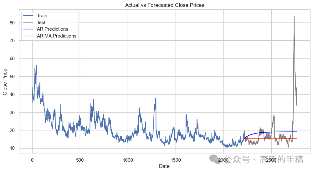
plt.figure(figsize=(12, 6))# Plot the actual valuesplt.plot(train.index, train, label='Train')plt.plot(test.index, test, label='Test', color='gray')# Plot the AR model forecastsplt.plot(test_ar.index, ar_predictions, label='AR Predictions', color='blue')# Plot the ARIMA model forecastsplt.plot(test_arima.index, arima_predictions, label='ARIMA Predictions', color='red')plt.xlabel('Date')plt.ylabel('Close Price')plt.title('Actual vs Forecasted Close Prices')plt.legend()plt.show()
发布者:股市刺客,转载请注明出处:https://www.95sca.cn/archives/111156
站内所有文章皆来自网络转载或读者投稿,请勿用于商业用途。如有侵权、不妥之处,请联系站长并出示版权证明以便删除。敬请谅解!


