
import numpy as npimport pandas as pdimport os, datetimeimport tensorflow as tffrom tensorflow.keras.models import *from tensorflow.keras.layers import *print('Tensorflow version: {}'.format(tf.__version__))import matplotlib.pyplot as pltplt.style.use('seaborn')import warningswarnings.filterwarnings('ignore')physical_devices = tf.config.list_physical_devices()print('Physical devices: {}'.format(physical_devices))# Filter out the CPUs and keep only the GPUsgpus = [device for device in physical_devices if 'GPU' in device.device_type]# If GPUs are available, set memory growth to Trueif len(gpus) > 0:tf.config.experimental.set_visible_devices(gpus[0], 'GPU')tf.config.experimental.set_memory_growth(gpus[0], True)print('GPU memory growth: True')
Tensorflow version: 2.9.1
Physical devices: [PhysicalDevice(name=’/physical_device:CPU:0′, device_type=’CPU’)]
Hyperparameters
batch_size = 32seq_len = 128d_k = 256d_v = 256n_heads = 12ff_dim = 256
Load IBM data
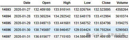
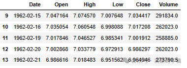
IBM_path = 'IBM.csv'df = pd.read_csv(IBM_path, delimiter=',', usecols=['Date', 'Open', 'High', 'Low', 'Close', 'Volume'])# Replace 0 to avoid dividing by 0 later ondf['Volume'].replace(to_replace=0, method='ffill', inplace=True)df.sort_values('Date', inplace=True)df.tail()
df.head()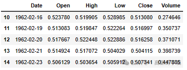
# print the shape of the datasetprint('Shape of the dataframe: {}'.format(df.shape))
Shape of the dataframe: (14588, 6)
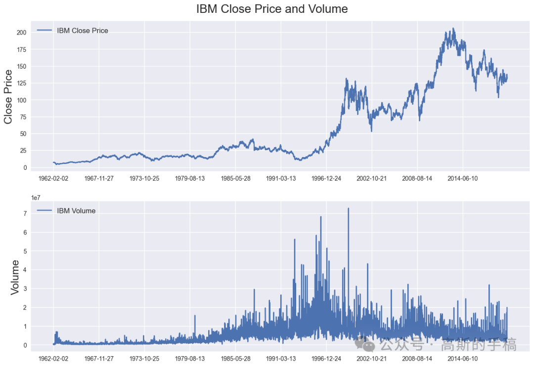
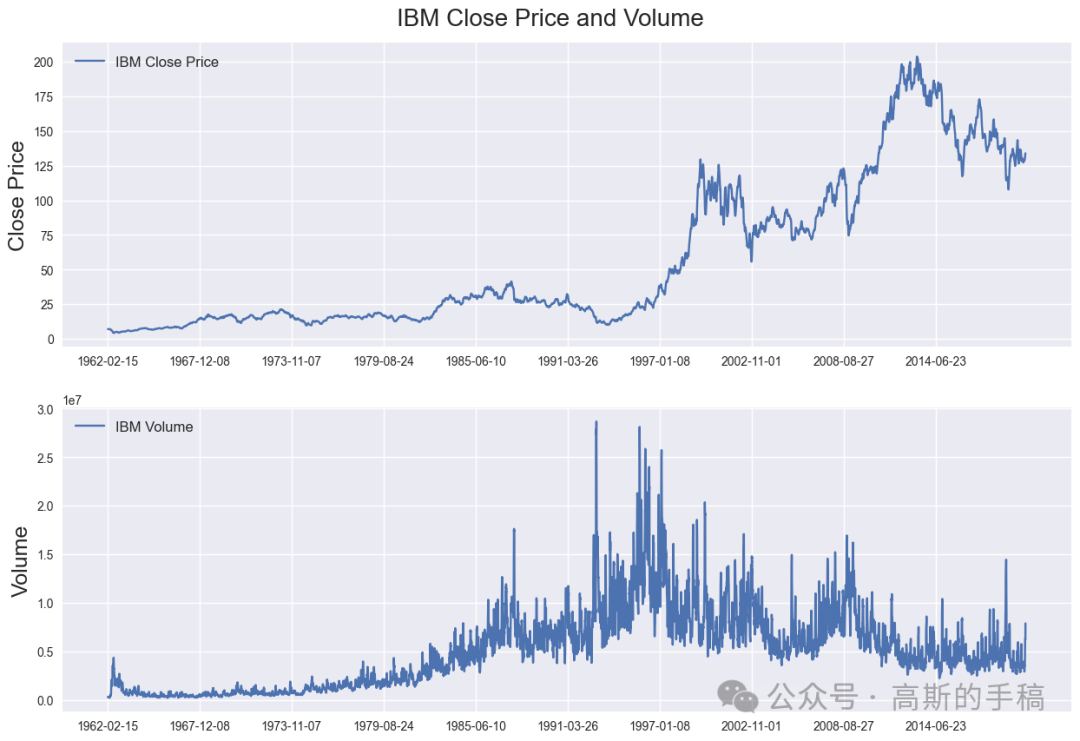
Plot daily IBM closing prices and volume
fig = plt.figure(figsize=(15,10))st = fig.suptitle("IBM Close Price and Volume", fontsize=20)st.set_y(0.92)ax1 = fig.add_subplot(211)ax1.plot(df['Close'], label='IBM Close Price')ax1.set_xticks(range(0, df.shape[0], 1464))ax1.set_xticklabels(df['Date'].loc[::1464])ax1.set_ylabel('Close Price', fontsize=18)ax1.legend(loc="upper left", fontsize=12)ax2 = fig.add_subplot(212)ax2.plot(df['Volume'], label='IBM Volume')ax2.set_xticks(range(0, df.shape[0], 1464))ax2.set_xticklabels(df['Date'].loc[::1464])ax2.set_ylabel('Volume', fontsize=18)ax2.legend(loc="upper left", fontsize=12)
Calculate normalized percentage change of all columns
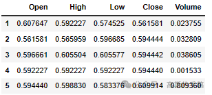
'''Calculate percentage change'''df['Open'] = df['Open'].pct_change() # Create arithmetic returns columndf['High'] = df['High'].pct_change() # Create arithmetic returns columndf['Low'] = df['Low'].pct_change() # Create arithmetic returns columndf['Close'] = df['Close'].pct_change() # Create arithmetic returns columndf['Volume'] = df['Volume'].pct_change()df.dropna(how='any', axis=0, inplace=True) # Drop all rows with NaN values###############################################################################'''Create indexes to split dataset'''times = sorted(df.index.values)last_10pct = sorted(df.index.values)[-int(0.1*len(times))] # Last 10% of serieslast_20pct = sorted(df.index.values)[-int(0.2*len(times))] # Last 20% of series###############################################################################'''Normalize price columns'''#min_return = min(df[(df.index < last_20pct)][['Open', 'High', 'Low', 'Close']].min(axis=0))max_return = max(df[(df.index < last_20pct)][['Open', 'High', 'Low', 'Close']].max(axis=0))# Min-max normalize price columns (0-1 range)df['Open'] = (df['Open'] - min_return) / (max_return - min_return)df['High'] = (df['High'] - min_return) / (max_return - min_return)df['Low'] = (df['Low'] - min_return) / (max_return - min_return)df['Close'] = (df['Close'] - min_return) / (max_return - min_return)###############################################################################'''Normalize volume column'''min_volume = df[(df.index < last_20pct)]['Volume'].min(axis=0)max_volume = df[(df.index < last_20pct)]['Volume'].max(axis=0)# Min-max normalize volume columns (0-1 range)df['Volume'] = (df['Volume'] - min_volume) / (max_volume - min_volume)###############################################################################'''Create training, validation and test split'''df_train = df[(df.index < last_20pct)] # Training data are 80% of total datadf_val = df[(df.index >= last_20pct) & (df.index < last_10pct)]df_test = df[(df.index >= last_10pct)]# Remove date columndf_train.drop(columns=['Date'], inplace=True)df_val.drop(columns=['Date'], inplace=True)df_test.drop(columns=['Date'], inplace=True)# Convert pandas columns into arraystrain_data = df_train.valuesval_data = df_val.valuestest_data = df_test.valuesprint('Training data shape: {}'.format(train_data.shape))print('Validation data shape: {}'.format(val_data.shape))print('Test data shape: {}'.format(test_data.shape))df_train.head()
Training data shape: (11678, 5)
Validation data shape: (1460, 5)
Test data shape: (1459, 5)
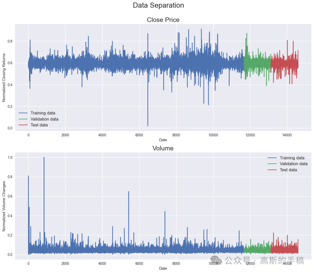
Plot daily changes of close prices and volume
fig = plt.figure(figsize=(15,12))st = fig.suptitle("Data Separation", fontsize=20)st.set_y(0.95)###############################################################################ax1 = fig.add_subplot(211)ax1.plot(np.arange(train_data.shape[0]), df_train['Close'], label='Training data')ax1.plot(np.arange(train_data.shape[0],train_data.shape[0]+val_data.shape[0]), df_val['Close'], label='Validation data')ax1.plot(np.arange(train_data.shape[0]+val_data.shape[0],train_data.shape[0]+val_data.shape[0]+test_data.shape[0]), df_test['Close'], label='Test data')ax1.set_xlabel('Date')ax1.set_ylabel('Normalized Closing Returns')ax1.set_title("Close Price", fontsize=18)ax1.legend(loc="best", fontsize=12)###############################################################################ax2 = fig.add_subplot(212)ax2.plot(np.arange(train_data.shape[0]), df_train['Volume'], label='Training data')ax2.plot(np.arange(train_data.shape[0],train_data.shape[0]+val_data.shape[0]), df_val['Volume'], label='Validation data')ax2.plot(np.arange(train_data.shape[0]+val_data.shape[0],train_data.shape[0]+val_data.shape[0]+test_data.shape[0]), df_test['Volume'], label='Test data')ax2.set_xlabel('Date')ax2.set_ylabel('Normalized Volume Changes')ax2.set_title("Volume", fontsize=18)ax2.legend(loc="best", fontsize=12)
Create chunks of training, validation and test data
# Training dataX_train, y_train = [], []for i in range(seq_len, len(train_data)):X_train.append(train_data[i-seq_len:i]) # Chunks of training data with a length of 128 df-rowsy_train.append(train_data[:, 3][i]) #Value of 4th column (Close Price) of df-row 128+1X_train, y_train = np.array(X_train), np.array(y_train)################################################################################ Validation dataX_val, y_val = [], []for i in range(seq_len, len(val_data)):X_val.append(val_data[i-seq_len:i])y_val.append(val_data[:, 3][i])X_val, y_val = np.array(X_val), np.array(y_val)################################################################################ Test dataX_test, y_test = [], []for i in range(seq_len, len(test_data)):X_test.append(test_data[i-seq_len:i])y_test.append(test_data[:, 3][i])X_test, y_test = np.array(X_test), np.array(y_test)print('Training set shape', X_train.shape, y_train.shape)print('Validation set shape', X_val.shape, y_val.shape)print('Testing set shape' ,X_test.shape, y_test.shape)
Training set shape (11550, 128, 5) (11550,)
Validation set shape (1332, 128, 5) (1332,)
Testing set shape (1331, 128, 5) (1331,)
TimeVector
class Time2Vector(Layer):def __init__(self, seq_len, **kwargs):super(Time2Vector, self).__init__()self.seq_len = seq_lendef build(self, input_shape):'''Initialize weights and biases with shape (batch, seq_len)'''self.weights_linear = self.add_weight(name='weight_linear',shape=(int(self.seq_len),),initializer='uniform',trainable=True)self.bias_linear = self.add_weight(name='bias_linear',shape=(int(self.seq_len),),initializer='uniform',trainable=True)self.weights_periodic = self.add_weight(name='weight_periodic',shape=(int(self.seq_len),),initializer='uniform',trainable=True)self.bias_periodic = self.add_weight(name='bias_periodic',shape=(int(self.seq_len),),initializer='uniform',trainable=True)def call(self, x):'''Calculate linear and periodic time features'''x = tf.math.reduce_mean(x[:,:,:4], axis=-1)time_linear = self.weights_linear * x + self.bias_linear # Linear time featuretime_linear = tf.expand_dims(time_linear, axis=-1) # Add dimension (batch, seq_len, 1)time_periodic = tf.math.sin(tf.multiply(x, self.weights_periodic) + self.bias_periodic)time_periodic = tf.expand_dims(time_periodic, axis=-1) # Add dimension (batch, seq_len, 1)return tf.concat([time_linear, time_periodic], axis=-1) # shape = (batch, seq_len, 2)def get_config(self): # Needed for saving and loading model with custom layerconfig = super().get_config().copy()config.update({'seq_len': self.seq_len})return config
Transformer
class SingleAttention(Layer):def __init__(self, d_k, d_v):super(SingleAttention, self).__init__()self.d_k = d_kself.d_v = d_vdef build(self, input_shape):self.query = Dense(self.d_k,input_shape=input_shape,kernel_initializer='glorot_uniform',bias_initializer='glorot_uniform')self.key = Dense(self.d_k,input_shape=input_shape,kernel_initializer='glorot_uniform',bias_initializer='glorot_uniform')self.value = Dense(self.d_v,input_shape=input_shape,kernel_initializer='glorot_uniform',bias_initializer='glorot_uniform')def call(self, inputs): # inputs = (in_seq, in_seq, in_seq)q = self.query(inputs[0])k = self.key(inputs[1])attn_weights = tf.matmul(q, k, transpose_b=True)attn_weights = tf.map_fn(lambda x: x/np.sqrt(self.d_k), attn_weights)attn_weights = tf.nn.softmax(attn_weights, axis=-1)v = self.value(inputs[2])attn_out = tf.matmul(attn_weights, v)return attn_out#############################################################################class MultiAttention(Layer):def __init__(self, d_k, d_v, n_heads):super(MultiAttention, self).__init__()self.d_k = d_kself.d_v = d_vself.n_heads = n_headsself.attn_heads = list()def build(self, input_shape):for n in range(self.n_heads):self.attn_heads.append(SingleAttention(self.d_k, self.d_v))# input_shape[0]=(batch, seq_len, 7), input_shape[0][-1]=7self.linear = Dense(input_shape[0][-1],input_shape=input_shape,kernel_initializer='glorot_uniform',bias_initializer='glorot_uniform')def call(self, inputs):attn = [self.attn_heads[i](inputs) for i in range(self.n_heads)]concat_attn = tf.concat(attn, axis=-1)multi_linear = self.linear(concat_attn)return multi_linear#############################################################################class TransformerEncoder(Layer):def __init__(self, d_k, d_v, n_heads, ff_dim, dropout=0.1, **kwargs):super(TransformerEncoder, self).__init__()self.d_k = d_kself.d_v = d_vself.n_heads = n_headsself.ff_dim = ff_dimself.attn_heads = list()self.dropout_rate = dropoutdef build(self, input_shape):self.attn_multi = MultiAttention(self.d_k, self.d_v, self.n_heads)self.attn_dropout = Dropout(self.dropout_rate)self.attn_normalize = LayerNormalization(input_shape=input_shape, epsilon=1e-6)self.ff_conv1D_1 = Conv1D(filters=self.ff_dim, kernel_size=1, activation='relu')# input_shape[0]=(batch, seq_len, 7), input_shape[0][-1] = 7self.ff_conv1D_2 = Conv1D(filters=input_shape[0][-1], kernel_size=1)self.ff_dropout = Dropout(self.dropout_rate)self.ff_normalize = LayerNormalization(input_shape=input_shape, epsilon=1e-6)def call(self, inputs): # inputs = (in_seq, in_seq, in_seq)attn_layer = self.attn_multi(inputs)attn_layer = self.attn_dropout(attn_layer)attn_layer = self.attn_normalize(inputs[0] + attn_layer)ff_layer = self.ff_conv1D_1(attn_layer)ff_layer = self.ff_conv1D_2(ff_layer)ff_layer = self.ff_dropout(ff_layer)ff_layer = self.ff_normalize(inputs[0] + ff_layer)return ff_layerdef get_config(self): # Needed for saving and loading model with custom layerconfig = super().get_config().copy()config.update({'d_k': self.d_k,'d_v': self.d_v,'n_heads': self.n_heads,'ff_dim': self.ff_dim,'attn_heads': self.attn_heads,'dropout_rate': self.dropout_rate})return config
Model
def create_model():'''Initialize time and transformer layers'''time_embedding = Time2Vector(seq_len)attn_layer1 = TransformerEncoder(d_k, d_v, n_heads, ff_dim)attn_layer2 = TransformerEncoder(d_k, d_v, n_heads, ff_dim)attn_layer3 = TransformerEncoder(d_k, d_v, n_heads, ff_dim)'''Construct model'''in_seq = Input(shape=(seq_len, 5))x = time_embedding(in_seq)x = Concatenate(axis=-1)([in_seq, x])x = attn_layer1((x, x, x))x = attn_layer2((x, x, x))x = attn_layer3((x, x, x))x = GlobalAveragePooling1D(data_format='channels_first')(x)x = Dropout(0.1)(x)x = Dense(64, activation='relu')(x)x = Dropout(0.1)(x)out = Dense(1, activation='linear')(x)model = Model(inputs=in_seq, outputs=out)model.compile(loss='mse', optimizer='adam', metrics=['mae', 'mape'])return modelmodel = create_model()model.summary()callback = tf.keras.callbacks.ModelCheckpoint('Transformer+TimeEmbedding.hdf5',monitor='val_loss',save_best_only=True, verbose=1)history = model.fit(X_train, y_train,batch_size=batch_size,epochs=35,callbacks=[callback],validation_data=(X_val, y_val))model = tf.keras.models.load_model('Transformer+TimeEmbedding.hdf5',custom_objects={'Time2Vector': Time2Vector,'SingleAttention': SingleAttention,'MultiAttention': MultiAttention,'TransformerEncoder': TransformerEncoder})###############################################################################'''Calculate predictions and metrics'''#Calculate predication for training, validation and test datatrain_pred = model.predict(X_train)val_pred = model.predict(X_val)test_pred = model.predict(X_test)#Print evaluation metrics for all datasetstrain_eval = model.evaluate(X_train, y_train, verbose=0)val_eval = model.evaluate(X_val, y_val, verbose=0)test_eval = model.evaluate(X_test, y_test, verbose=0)print(' ')print('Evaluation metrics')print('Training Data - Loss: {:.4f}, MAE: {:.4f}, MAPE: {:.4f}'.format(train_eval[0], train_eval[1], train_eval[2]))print('Validation Data - Loss: {:.4f}, MAE: {:.4f}, MAPE: {:.4f}'.format(val_eval[0], val_eval[1], val_eval[2]))print('Test Data - Loss: {:.4f}, MAE: {:.4f}, MAPE: {:.4f}'.format(test_eval[0], test_eval[1], test_eval[2]))###############################################################################'''Display results'''fig = plt.figure(figsize=(15,20))st = fig.suptitle("Transformer + TimeEmbedding Model", fontsize=22)st.set_y(0.92)#Plot training data resultsax11 = fig.add_subplot(311)ax11.plot(train_data[:, 3], label='IBM Closing Returns')ax11.plot(np.arange(seq_len, train_pred.shape[0]+seq_len), train_pred, linewidth=3, label='Predicted IBM Closing Returns')ax11.set_title("Training Data", fontsize=18)ax11.set_xlabel('Date')ax11.set_ylabel('IBM Closing Returns')ax11.legend(loc="best", fontsize=12)#Plot validation data resultsax21 = fig.add_subplot(312)ax21.plot(val_data[:, 3], label='IBM Closing Returns')ax21.plot(np.arange(seq_len, val_pred.shape[0]+seq_len), val_pred, linewidth=3, label='Predicted IBM Closing Returns')ax21.set_title("Validation Data", fontsize=18)ax21.set_xlabel('Date')ax21.set_ylabel('IBM Closing Returns')ax21.legend(loc="best", fontsize=12)#Plot test data resultsax31 = fig.add_subplot(313)ax31.plot(test_data[:, 3], label='IBM Closing Returns')ax31.plot(np.arange(seq_len, test_pred.shape[0]+seq_len), test_pred, linewidth=3, label='Predicted IBM Closing Returns')ax31.set_title("Test Data", fontsize=18)ax31.set_xlabel('Date')ax31.set_ylabel('IBM Closing Returns')ax31.legend(loc="best", fontsize=12)
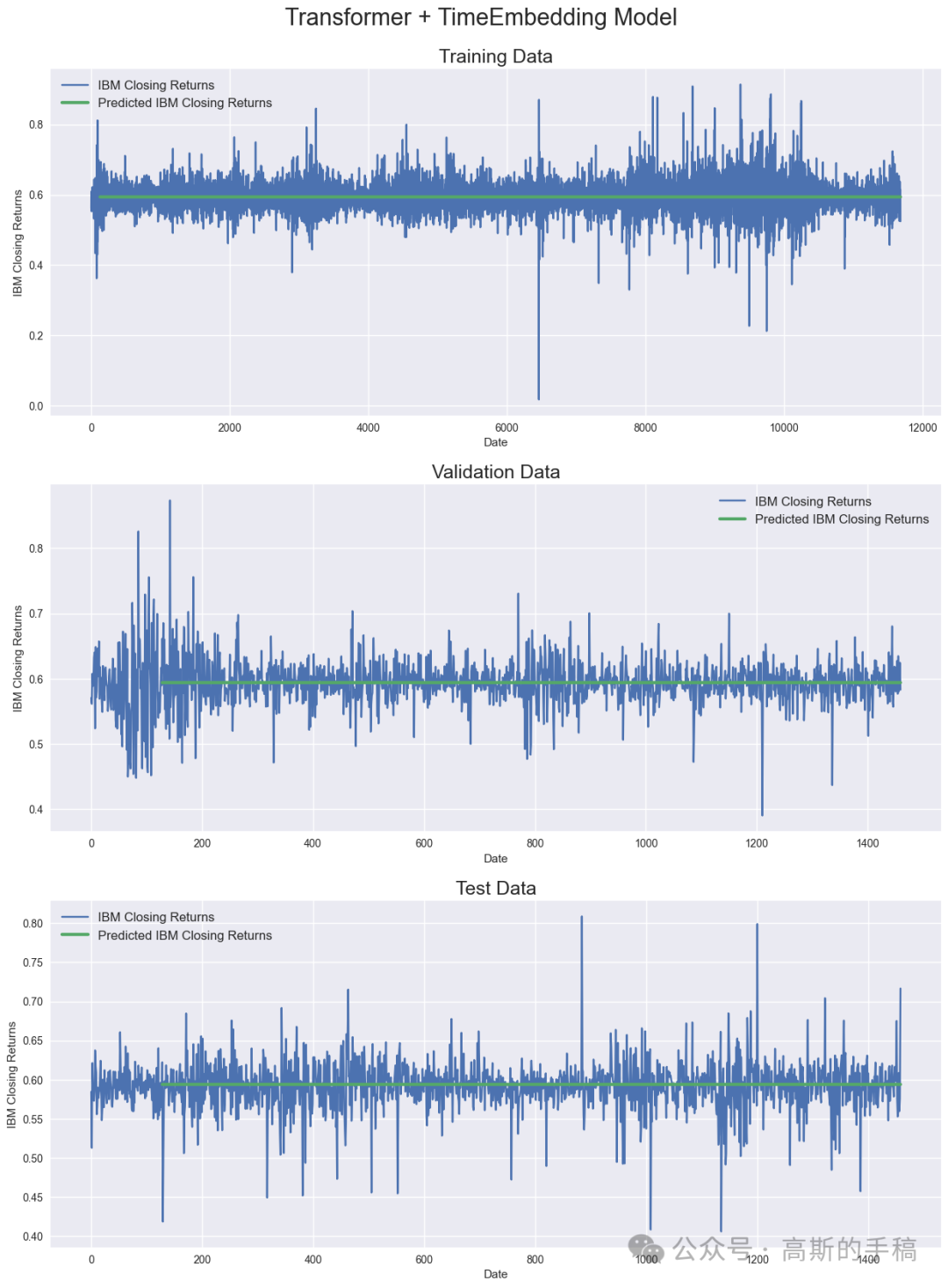
###############################################################################'''Calculate predictions and metrics'''#Calculate predication for training, validation and test datatrain_pred = model.predict(X_train)val_pred = model.predict(X_val)test_pred = model.predict(X_test)#Print evaluation metrics for all datasetstrain_eval = model.evaluate(X_train, y_train, verbose=0)val_eval = model.evaluate(X_val, y_val, verbose=0)test_eval = model.evaluate(X_test, y_test, verbose=0)print(' ')print('Evaluation metrics')print('Training Data - Loss: {:.4f}, MAE: {:.4f}, MAPE: {:.4f}'.format(train_eval[0], train_eval[1], train_eval[2]))print('Validation Data - Loss: {:.4f}, MAE: {:.4f}, MAPE: {:.4f}'.format(val_eval[0], val_eval[1], val_eval[2]))print('Test Data - Loss: {:.4f}, MAE: {:.4f}, MAPE: {:.4f}'.format(test_eval[0], test_eval[1], test_eval[2]))###############################################################################'''Display results'''fig = plt.figure(figsize=(15,20))st = fig.suptitle("Transformer + TimeEmbedding Model", fontsize=22)st.set_y(0.92)#Plot training data resultsax11 = fig.add_subplot(311)ax11.plot(train_data[:, 3], label='IBM Closing Returns')ax11.plot(np.arange(seq_len, train_pred.shape[0]+seq_len), train_pred, linewidth=3, label='Predicted IBM Closing Returns')ax11.set_title("Training Data", fontsize=18)ax11.set_xlabel('Date')ax11.set_ylabel('IBM Closing Returns')ax11.legend(loc="best", fontsize=12)#Plot validation data resultsax21 = fig.add_subplot(312)ax21.plot(val_data[:, 3], label='IBM Closing Returns')ax21.plot(np.arange(seq_len, val_pred.shape[0]+seq_len), val_pred, linewidth=3, label='Predicted IBM Closing Returns')ax21.set_title("Validation Data", fontsize=18)ax21.set_xlabel('Date')ax21.set_ylabel('IBM Closing Returns')ax21.legend(loc="best", fontsize=12)#Plot test data resultsax31 = fig.add_subplot(313)ax31.plot(test_data[:, 3], label='IBM Closing Returns')ax31.plot(np.arange(seq_len, test_pred.shape[0]+seq_len), test_pred, linewidth=3, label='Predicted IBM Closing Returns')ax31.set_title("Test Data", fontsize=18)ax31.set_xlabel('Date')ax31.set_ylabel('IBM Closing Returns')ax31.legend(loc="best", fontsize=12)
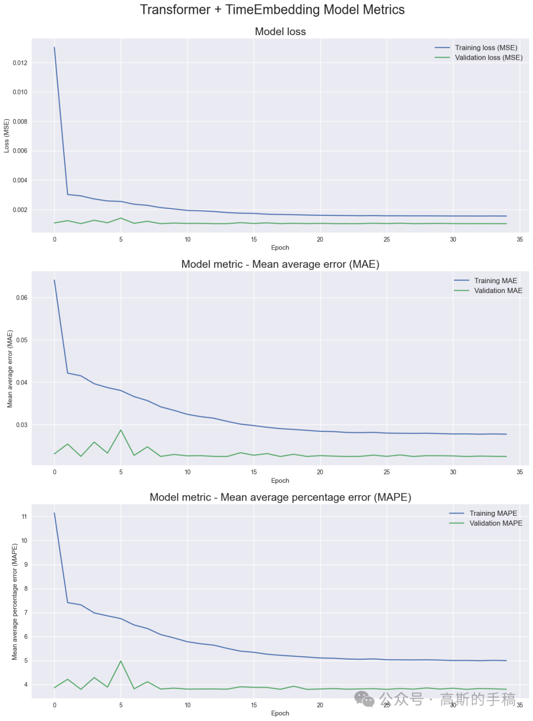
Model metrics
'''Display model metrics'''fig = plt.figure(figsize=(15,20))st = fig.suptitle("Transformer + TimeEmbedding Model Metrics", fontsize=22)st.set_y(0.92)#Plot model lossax1 = fig.add_subplot(311)ax1.plot(history.history['loss'], label='Training loss (MSE)')ax1.plot(history.history['val_loss'], label='Validation loss (MSE)')ax1.set_title("Model loss", fontsize=18)ax1.set_xlabel('Epoch')ax1.set_ylabel('Loss (MSE)')ax1.legend(loc="best", fontsize=12)#Plot MAEax2 = fig.add_subplot(312)ax2.plot(history.history['mae'], label='Training MAE')ax2.plot(history.history['val_mae'], label='Validation MAE')ax2.set_title("Model metric - Mean average error (MAE)", fontsize=18)ax2.set_xlabel('Epoch')ax2.set_ylabel('Mean average error (MAE)')ax2.legend(loc="best", fontsize=12)#Plot MAPEax3 = fig.add_subplot(313)ax3.plot(history.history['mape'], label='Training MAPE')ax3.plot(history.history['val_mape'], label='Validation MAPE')ax3.set_title("Model metric - Mean average percentage error (MAPE)", fontsize=18)ax3.set_xlabel('Epoch')ax3.set_ylabel('Mean average percentage error (MAPE)')ax3.legend(loc="best", fontsize=12)
Model architecture overview
tf.keras.utils.plot_model(model,to_file="IBM_Transformer+TimeEmbedding.png",show_shapes=True,show_layer_names=True,expand_nested=True,dpi=96,)
tf.keras.utils.plot_model(model,to_file="IBM_Transformer+TimeEmbedding.png",show_shapes=True,show_layer_names=True,expand_nested=True,dpi=96,)
Moving Average
Moving Average – Load IBM data again, to apply rolling window
IBM_path = 'IBM.csv'df = pd.read_csv(IBM_path, delimiter=',', usecols=['Date', 'Open', 'High', 'Low', 'Close', 'Volume'])# Replace 0 to avoid dividing by 0 later ondf['Volume'].replace(to_replace=0, method='ffill', inplace=True)df.sort_values('Date', inplace=True)# Apply moving average with a window of 10 days to all columnsdf[['Open', 'High', 'Low', 'Close', 'Volume']] = df[['Open', 'High', 'Low', 'Close', 'Volume']].rolling(10).mean()# Drop all rows with NaN valuesdf.dropna(how='any', axis=0, inplace=True)df.head()
Moving Average – Plot daily IBM closing prices and volume
fig = plt.figure(figsize=(15,10))st = fig.suptitle("IBM Close Price and Volume", fontsize=20)st.set_y(0.92)ax1 = fig.add_subplot(211)ax1.plot(df['Close'], label='IBM Close Price')ax1.set_xticks(range(0, df.shape[0], 1464))ax1.set_xticklabels(df['Date'].loc[::1464])ax1.set_ylabel('Close Price', fontsize=18)ax1.legend(loc="upper left", fontsize=12)ax2 = fig.add_subplot(212)ax2.plot(df['Volume'], label='IBM Volume')ax2.set_xticks(range(0, df.shape[0], 1464))ax2.set_xticklabels(df['Date'].loc[::1464])ax2.set_ylabel('Volume', fontsize=18)ax2.legend(loc="upper left", fontsize=12)
发布者:股市刺客,转载请注明出处:https://www.95sca.cn/archives/111157
站内所有文章皆来自网络转载或读者投稿,请勿用于商业用途。如有侵权、不妥之处,请联系站长并出示版权证明以便删除。敬请谅解!


