基于简单时间序列分析的股票价格预测（Python）

pip install pmdarima

import numpy as npimport pandas as pdimport matplotlib.pyplot as pltfrom pandas.plotting import lag_plotfrom pandas.plotting import autocorrelation_plotfrom datetime import datefrom statsmodels.tsa.stattools import adfullerfrom statsmodels.tsa.seasonal import seasonal_decomposefrom statsmodels.tsa.arima.model import ARIMAfrom sklearn.metrics import mean_squared_errorfrom pandas.plotting import register_matplotlib_convertersfrom pmdarima.arima import ADFTestregister_matplotlib_converters()
df = pd.read_csv('Tesla.csv')print(df.head(5))

 Date      Open      High       Low     Close  Adj Close     Volume
0  29/06/2010  1.266667  1.666667  1.169333  1.592667   1.592667  281494500
1  30/06/2010  1.719333  2.028000  1.553333  1.588667   1.588667  257806500
2  01/07/2010  1.666667  1.728000  1.351333  1.464000   1.464000  123282000
3  02/07/2010  1.533333  1.540000  1.247333  1.280000   1.280000   77097000
4  06/07/2010  1.333333  1.333333  1.055333  1.074000   1.074000  103003500

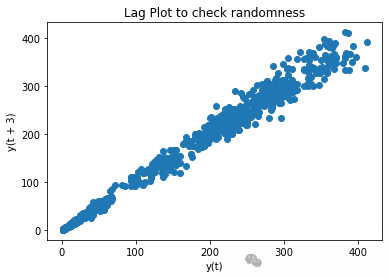
plt.figure()lag_plot(df['Open'],lag=3)plt.title('Lag Plot to check randomness')plt.show

plt.figure(figsize=(20, 10))plt.plot(df["Date"],df["Close"])plt.xticks(np.arange(0,3500,500),df['Date'][0:3500:500],rotation='vertical')plt.title("Tesla stock price over time")plt.xlabel("TIME")plt.ylabel("PRICE")plt.show

adf_test=ADFTest(alpha = 0.05)adf_test.should_diff(df['Close'])

result = seasonal_decompose(df["Close"],                            model='multiplicative', period = 30)fig = plt.figure()fig = result.plot()fig.set_size_inches(15, 10)

from statsmodels.tsa.stattools import adfullerdef test_stationarity(timeseries, window = 12):
    #Determing rolling statistics    rolmean = timeseries.rolling(window).mean()    rolstd = timeseries.rolling(window).std()
    #Plot rolling statistics:    fig = plt.figure(figsize=(12, 8))    orig = plt.plot(timeseries, color='blue',label='Original')    mean = plt.plot(rolmean, color='red', label='Rolling Mean')    std = plt.plot(rolstd, color='black', label = 'Rolling Std')    plt.legend(loc='best')    plt.title('Rolling Mean & Standard Deviation')    plt.show()    #Perform Dickey-Fuller test:    print('Results of Dickey-Fuller Test:')    dftest = adfuller(timeseries, autolag='AIC', maxlag = 20 )    dfoutput = pd.Series(dftest[0:4], index=['Test Statistic','p-value','#Lags Used','Number of Observations Used'])    for key,value in dftest[4].items():        dfoutput['Critical Value (%s)'%key] = value    pvalue = dftest[1]    if pvalue < 0.05:        print('p-value = %.4f. The series is likely stationary.' % pvalue)    else:        print('p-value = %.4f. The series is likely non-stationary.' % pvalue)
    print(dfoutput)

test_stationarity(df['Close'])

first_diff = df.Close - df.Close.shift(1)first_diff = first_diff.dropna(inplace = False)test_stationarity(first_diff, window = 12)

train_data, test_data = df[0:int(len(df)*0.7)], df[int(len(df)*0.7):]training_data = train_data['Close'].valuestest_data = test_data['Close'].valueshistory = [x for x in training_data]model_predictions = []N_test_observations = len(test_data)for time_point in range(N_test_observations):    model = ARIMA(history, order=(4,1,0))    model_fit = model.fit()    output = model_fit.forecast()    yhat = output[0]    model_predictions.append(yhat)    true_test_value = test_data[time_point]    history.append(true_test_value)MSE_error = mean_squared_error(test_data, model_predictions)print('Testing Mean Squared Error is {}'.format(MSE_error))print(model_fit.summary())

Testing Mean Squared Error is 66.13403523914238
                               SARIMAX Results                                
==============================================================================
Dep. Variable:                      y   No. Observations:                 3164
Model:                 ARIMA(4, 1, 0)   Log Likelihood               -9183.629
Date:                Mon, 30 Jan 2023   AIC                          18377.257
Time:                        04:11:07   BIC                          18407.554
Sample:                             0   HQIC                         18388.126
                               - 3164                                         
Covariance Type:                  opg                                         
==============================================================================
                 coef    std err          z      P>|z|      [0.025      0.975]
------------------------------------------------------------------------------
ar.L1         -0.0380      0.008     -4.899      0.000      -0.053      -0.023
ar.L2          0.0154      0.007      2.335      0.020       0.002       0.028
ar.L3         -0.0002      0.009     -0.024      0.981      -0.017       0.017
ar.L4          0.0407      0.007      5.747      0.000       0.027       0.055
sigma2        19.4734      0.136    143.711      0.000      19.208      19.739
===================================================================================
Ljung-Box (L1) (Q):                   0.00   Jarque-Bera (JB):             80170.86
Prob(Q):                              0.98   Prob(JB):                         0.00
Heteroskedasticity (H):            1019.90   Skew:                            -0.15
Prob(H) (two-sided):                  0.00   Kurtosis:                        27.66
===================================================================================

Warnings:
[1] Covariance matrix calculated using the outer product of gradients (complex-step).

test_set_range = df[int(len(df)*0.7):].indexplt.figure(figsize=(20, 10))plt.plot(test_set_range, model_predictions, color='blue', marker='o', linestyle='dashed',label='Predicted Price')plt.plot(test_set_range, test_data, color='red', label='Actual Price')plt.title('TESLA Prices Prediction')plt.xlabel('Date')plt.ylabel('Prices')plt.xticks(np.arange(2200,3146,100), df.Date[2200:3146:100],rotation='vertical')plt.legend()plt.show()