
Step 1: Loading the data
import numpy as npimport pandas as pdimport matplotlib.pyplot as pltimport torch.nn as nnimport torchfrom torch.autograd import Variablefrom torch.utils.data import Dataset, DataLoader
# Importing the training setdataset = pd.read_csv('HistoricalData_1719412320530.csv')
dataset.head(10)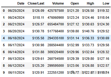
dataset.info()<class 'pandas.core.frame.DataFrame'> RangeIndex: 2516 entries, 0 to 2515 Data columns (total 6 columns): # Column Non-Null Count Dtype --- ------ -------------- ----- 0 Date 2516 non-null object 1 Close/Last 2516 non-null object 2 Volume 2516 non-null int64 3 Open 2516 non-null object 4 High 2516 non-null object 5 Low 2516 non-null object dtypes: int64(1), object(5) memory usage: 118.1+ KB
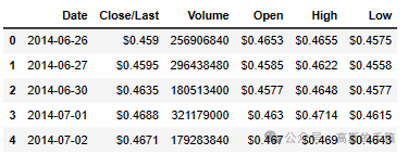
dataset['Date'] = pd.to_datetime(dataset['Date'], format='%m/%d/%Y')dataset = dataset.sort_values(by='Date', ascending=True)dataset = dataset.reset_index(drop=True)
dataset.head(5)
dataset['Close/Last'] = dataset['Close/Last'].str.replace('dataset.head(5)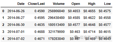
dataset_cl = dataset['Close/Last'].values# Feature Scalingfrom sklearn.preprocessing import MinMaxScalersc = MinMaxScaler(feature_range = (0, 1))# scale the datadataset_cl = dataset_cl.reshape(dataset_cl.shape[0], 1)dataset_cl = sc.fit_transform(dataset_cl)dataset_cl
array([[2.91505500e-04],
       [2.95204809e-04],
       [3.24799276e-04],
       ...,
       [9.33338463e-01],
       [8.70746165e-01],
       [9.29787127e-01]])
Step 2: Cutting time series into sequences (Sliding Window)
input_size = 7# Create a function to process the data into 7 day look back slices# lb is window sizedef processData(data, lb):X, y = [], [] # X is input vector, Y is output vectorfor i in range(len(data) - lb - 1):X.append(data[i: (i + lb), 0])y.append(data[(i + lb), 0])return np.array(X), np.array(y)X, y = processData(dataset_cl, input_size)
Step 3: Split training and testing sets
X_train, X_test = X[:int(X.shape[0]*0.80)], X[int(X.shape[0]*0.80):]y_train, y_test = y[:int(y.shape[0]*0.80)], y[int(y.shape[0]*0.80):]print(X_train.shape[0])print(X_test.shape[0])print(y_train.shape[0])print(y_test.shape[0])# reshapingX_train = np.reshape(X_train, (X_train.shape[0], 1, X_train.shape[1]))X_test = np.reshape(X_test, (X_test.shape[0], 1, X_test.shape[1]))
2006
502
2006
502
Step 4: Build and run an RNN regression model
class RNN(nn.Module):def __init__(self, i_size, h_size, n_layers, o_size, dropout=0.1, bidirectional=False):super().__init__()# super(RNN, self).__init__()self.num_directions = bidirectional + 1# LSTM moduleself.rnn = nn.LSTM(input_size = i_size,hidden_size = h_size,num_layers = n_layers,dropout = dropout,bidirectional = bidirectional)# self.relu = nn.ReLU()# Output layerself.out = nn.Linear(h_size, o_size)def forward(self, x, h_state):# r_out contains the LSTM output at each time step, and hidden_state# contains the hidden and cell states after processing the entire sequence.r_out, hidden_state = self.rnn(x, h_state)hidden_size = hidden_state[-1].size(-1)# Convert dimension of r_out (-1 denotes it depends on other parameters)r_out = r_out.view(-1, self.num_directions, hidden_size)# r_out = self.relu(r_out)outs = self.out(r_out)return outs, hidden_state
# Global settingINPUT_SIZE = input_size # LSTM input sizeHIDDEN_SIZE = 256NUM_LAYERS = 3 # LSTM 'stack' layerOUTPUT_SIZE = 1# Hyper parameterslearning_rate = 0.001num_epochs = 300rnn = RNN(INPUT_SIZE, HIDDEN_SIZE, NUM_LAYERS, OUTPUT_SIZE, bidirectional=False)rnn.cuda()optimiser = torch.optim.Adam(rnn.parameters(), lr=learning_rate)criterion = nn.MSELoss()hidden_state = None
rnnRNN( (rnn): LSTM(7, 256, num_layers=3, dropout=0.1) (out): Linear(in_features=256, out_features=1, bias=True) )
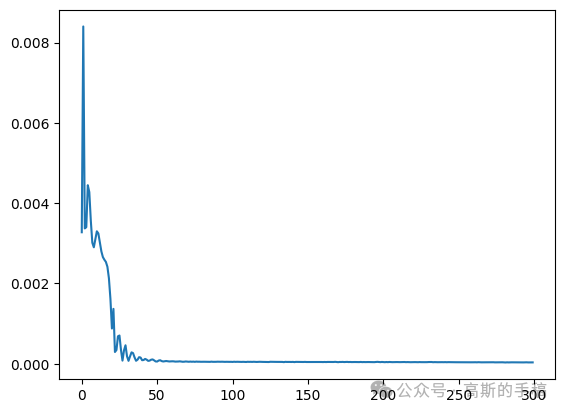
history = [] # save loss in each epoch# .cuda() copies element to the GPU memoryX_test_cuda = torch.tensor(X_test).float().cuda()y_test_cuda = torch.tensor(y_test).float().cuda()# Use all the data in one batchinputs_cuda = torch.tensor(X_train).float().cuda()labels_cuda = torch.tensor(y_train).float().cuda()# trainingfor epoch in range(num_epochs):# Train modernn.train()output, _ = rnn(inputs_cuda, hidden_state)# print(output.size())loss = criterion(output[:,0,:].view(-1), labels_cuda)optimiser.zero_grad()loss.backward() # back propagationoptimiser.step() # update the parametersif epoch % 20 == 0:# Convert train mode to evaluation mode (disable dropout)rnn.eval()test_output, _ = rnn(X_test_cuda, hidden_state)test_loss = criterion(test_output.view(-1), y_test_cuda)print('epoch {}, loss {}, eval loss {}'.format(epoch, loss.item(), test_loss.item()))else:print('epoch {}, loss {}'.format(epoch, loss.item()))history.append(loss.item())
# iterate over all the learnable parameters in the model, which include the# weights and biases of all layers in the model# (both the LSTM layers and the final linear layer)for param in rnn.parameters():print(param.data)
Step 5: Checking model performance
plt.plot(history)# dplt.plot(history.history['val_loss'])
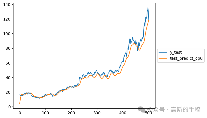
# X_train_X_test = np.concatenate((X_train, X_test),axis=0)# hidden_state = Nonernn.eval()# test_inputs = torch.tensor(X_test).float().cuda()test_predict, _ = rnn(X_test_cuda, hidden_state)test_predict_cpu = test_predict.cpu().detach().numpy()
plt.plot(sc.inverse_transform(y_test.reshape(-1,1)))plt.plot(sc.inverse_transform(test_predict_cpu.reshape(-1,1)))plt.legend(['y_test','test_predict_cpu'], loc='center left', bbox_to_anchor=(1, 0.5))
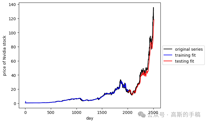
# plot original dataplt.plot(sc.inverse_transform(y.reshape(-1,1)), color='k')# train_inputs = torch.tensor(X_train).float().cuda()train_pred, hidden_state = rnn(inputs_cuda, None)train_pred_cpu = train_pred.cpu().detach().numpy()# use hidden state from previous training datatest_predict, _ = rnn(X_test_cuda, hidden_state)test_predict_cpu = test_predict.cpu().detach().numpy()# plt.plot(scl.inverse_transform(y_test.reshape(-1,1)))split_pt = int(X.shape[0] * 0.80) + 7 # window_sizeplt.plot(np.arange(7, split_pt, 1), sc.inverse_transform(train_pred_cpu.reshape(-1,1)), color='b')plt.plot(np.arange(split_pt, split_pt + len(test_predict_cpu), 1), sc.inverse_transform(test_predict_cpu.reshape(-1,1)), color='r')# pretty up graphplt.xlabel('day')plt.ylabel('price of Nvidia stock')plt.legend(['original series','training fit','testing fit'], loc='center left', bbox_to_anchor=(1, 0.5))plt.show()
MMSE = np.sum((test_predict_cpu.reshape(1,X_test.shape[0])-y[2006:])**2)/X_test.shape[0]print(MMSE)
0.0018420128176938062
, ”).astype(float)
Step 2: Cutting time series into sequences (Sliding Window)
Step 3: Split training and testing sets
Step 4: Build and run an RNN regression model
Step 5: Checking model performance
发布者:股市刺客,转载请注明出处:https://www.95sca.cn/archives/111154
站内所有文章皆来自网络转载或读者投稿,请勿用于商业用途。如有侵权、不妥之处,请联系站长并出示版权证明以便删除。敬请谅解!


