
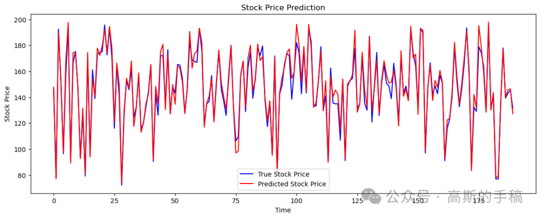
import yfinance as yfimport numpy as npimport pandas as pdfrom sklearn.preprocessing import MinMaxScalerfrom sklearn.model_selection import train_test_splitfrom sklearn.metrics import mean_absolute_error, mean_squared_error, mean_absolute_percentage_errorimport tensorflow as tffrom tensorflow.keras.models import Sequentialfrom tensorflow.keras.layers import Conv2D, MaxPooling2D, LSTM, Dense, Flattenimport matplotlib.pyplot as plt# Fetch stock dataticker = 'AAPL' # You can replace 'AAPL' with any ticker symboldata = yf.download(ticker, start='2020-01-01', end='2023-12-31')# Assuming 'Close' column contains the stock pricesprices = data['Close'].values.reshape(-1, 1)# Normalize the datascaler = MinMaxScaler(feature_range=(0, 1))scaled_prices = scaler.fit_transform(prices)# Create sequencesdef create_sequences(data, seq_length):X = []y = []for i in range(len(data) - seq_length):X.append(data[i:i + seq_length])y.append(data[i + seq_length])return np.array(X), np.array(y)seq_length = 60 # Number of past days to consider for predicting the next day's priceX, y = create_sequences(scaled_prices, seq_length)# Split into training and testing setsX_train, X_test, y_train, y_test = train_test_split(X, y, test_size=0.2, random_state=42)# Reshape for CNN inputX_train = X_train.reshape(X_train.shape[0], X_train.shape[1], 1, 1)X_test = X_test.reshape(X_test.shape[0], X_test.shape[1], 1, 1)# Define the modelmodel = Sequential()model.add(Conv2D(filters=64, kernel_size=(2, 1), activation='relu', input_shape=(seq_length, 1, 1)))model.add(MaxPooling2D(pool_size=(2, 1)))model.add(Flatten())model.add(tf.keras.layers.Reshape((29, 64)))model.add(LSTM(units=50, return_sequences=True))model.add(LSTM(units=50))model.add(Dense(units=1))# Compile the modelmodel.compile(optimizer='adam', loss='mean_squared_error')# Train the modelhistory = model.fit(X_train, y_train, epochs=50, batch_size=32, validation_data=(X_test, y_test))# Evaluate the modelloss = model.evaluate(X_test, y_test)print(f'Test Loss: {loss}')# Predict and inverse transform the predictionspredicted_prices = model.predict(X_test)predicted_prices = scaler.inverse_transform(predicted_prices)# Inverse transform the true pricestrue_prices = scaler.inverse_transform(y_test)# Calculate metricsmae = mean_absolute_error(true_prices, predicted_prices)rmse = np.sqrt(mean_squared_error(true_prices, predicted_prices))mape = mean_absolute_percentage_error(true_prices, predicted_prices)print(f'Mean Absolute Error (MAE): {mae}')print(f'Root Mean Squared Error (RMSE): {rmse}')print(f'Mean Absolute Percentage Error (MAPE): {mape}')# Calculate accuracydef calculate_accuracy(y_true, y_pred, tolerance=0.05):accurate_predictions = np.abs((y_true - y_pred) / y_true) < toleranceaccuracy = np.mean(accurate_predictions) * 100return accuracyaccuracy = calculate_accuracy(true_prices, predicted_prices)print(f'Accuracy: {accuracy:.2f}%')# Plot the resultsplt.figure(figsize=(14, 5))plt.plot(true_prices, color='blue', label='True Stock Price')plt.plot(predicted_prices, color='red', label='Predicted Stock Price')plt.title('Stock Price Prediction')plt.xlabel('Time')plt.ylabel('Stock Price')plt.legend()plt.show()
import yfinance as yfimport numpy as npimport pandas as pdfrom sklearn.preprocessing import MinMaxScalerfrom sklearn.model_selection import train_test_splitfrom sklearn.metrics import mean_absolute_error, mean_squared_error, mean_absolute_percentage_errorimport tensorflow as tffrom tensorflow.keras.models import Sequentialfrom tensorflow.keras.layers import Conv2D, MaxPooling2D, LSTM, Dense, Flattenimport matplotlib.pyplot as plt# Fetch stock dataticker = 'AAPL' # You can replace 'AAPL' with any ticker symboldata = yf.download(ticker, start='2020-01-01', end='2023-12-31')# Use multiple features: 'Open', 'High', 'Low', 'Close', 'Volume'features = data[['Open', 'High', 'Low', 'Close', 'Volume']]# Normalize the datascaler = MinMaxScaler(feature_range=(0, 1))scaled_features = scaler.fit_transform(features)# Create sequencesdef create_sequences(data, seq_length):X = []y = []for i in range(len(data) - seq_length):X.append(data[i:i + seq_length])y.append(data[i + seq_length, 3]) # Using the 'Close' price as the targetreturn np.array(X), np.array(y)seq_length = 60 # Number of past days to consider for predicting the next day's priceX, y = create_sequences(scaled_features, seq_length)# Split into training and testing setsX_train, X_test, y_train, y_test = train_test_split(X, y, test_size=0.2, random_state=42)# Reshape for CNN input (Adding an extra dimension for the single channel)X_train = X_train.reshape(X_train.shape[0], X_train.shape[1], X_train.shape[2], 1)X_test = X_test.reshape(X_test.shape[0], X_test.shape[1], X_test.shape[2], 1)# Define the modelmodel = Sequential()model.add(Conv2D(filters=64, kernel_size=(2, 5), activation='relu', input_shape=(seq_length, X_train.shape[2], 1)))model.add(MaxPooling2D(pool_size=(2, 1)))model.add(Flatten())model.add(tf.keras.layers.Reshape((29, 64)))model.add(LSTM(units=50, return_sequences=True))model.add(LSTM(units=50))model.add(Dense(units=1))# Compile the modelmodel.compile(optimizer='adam', loss='mean_squared_error')# Train the modelhistory = model.fit(X_train, y_train, epochs=50, batch_size=32, validation_data=(X_test, y_test))# Evaluate the modelloss = model.evaluate(X_test, y_test)print(f'Test Loss: {loss}')# Predict and inverse transform the predictionspredicted_prices = model.predict(X_test)predicted_prices = scaler.inverse_transform(np.hstack((np.zeros((predicted_prices.shape[0], 3)), predicted_prices, np.zeros((predicted_prices.shape[0], 1)))))[:, 3]# Inverse transform the true pricestrue_prices = scaler.inverse_transform(np.hstack((np.zeros((y_test.shape[0], 3)), y_test.reshape(-1, 1), np.zeros((y_test.shape[0], 1)))))[:, 3]# Calculate metricsmae = mean_absolute_error(true_prices, predicted_prices)rmse = np.sqrt(mean_squared_error(true_prices, predicted_prices))mape = mean_absolute_percentage_error(true_prices, predicted_prices)print(f'Mean Absolute Error (MAE): {mae}')print(f'Root Mean Squared Error (RMSE): {rmse}')print(f'Mean Absolute Percentage Error (MAPE): {mape}')# Calculate accuracydef calculate_accuracy(y_true, y_pred, tolerance=0.05):accurate_predictions = np.abs((y_true - y_pred) / y_true) < toleranceaccuracy = np.mean(accurate_predictions) * 100return accuracyaccuracy = calculate_accuracy(true_prices, predicted_prices)print(f'Accuracy: {accuracy:.2f}%')# Plot the resultsplt.figure(figsize=(14, 5))plt.plot(true_prices, color='blue', label='True Stock Price')plt.plot(predicted_prices, color='red', label='Predicted Stock Price')plt.title('Stock Price Prediction')plt.xlabel('Time')plt.ylabel('Stock Price')plt.legend()plt.show()
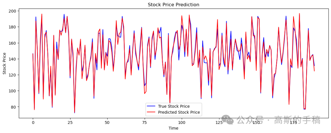
import yfinance as yfimport numpy as npimport pandas as pdfrom sklearn.preprocessing import MinMaxScalerfrom sklearn.model_selection import train_test_splitfrom sklearn.metrics import mean_absolute_error, mean_squared_error, mean_absolute_percentage_errorimport tensorflow as tffrom tensorflow.keras.models import Sequentialfrom tensorflow.keras.layers import Conv2D, MaxPooling2D, LSTM, Dense, Flattenimport matplotlib.pyplot as plt# Fetch stock dataticker = 'AAPL' # You can replace 'AAPL' with any ticker symboldata = yf.download(ticker, start='2020-01-01', end='2023-12-31')# Calculate additional featuresdata['SMA'] = data['Close'].rolling(window=20).mean() # Simple Moving Averagedata['EWMA'] = data['Close'].ewm(span=20, adjust=False).mean() # Exponential Moving Averagedata['Momentum'] = data['Close'] - data['Close'].shift(4) # Momentumdata['Volatility'] = data['Close'].rolling(window=20).std() # Rolling volatilitydata.dropna(inplace=True)# Use multiple features: 'Open', 'High', 'Low', 'Close', 'Volume', 'SMA', 'EWMA', 'Momentum', 'Volatility'features = data[['Open', 'High', 'Low', 'Close', 'Volume', 'SMA', 'EWMA', 'Momentum', 'Volatility']]# Normalize the datascaler = MinMaxScaler(feature_range=(0, 1))scaled_features = scaler.fit_transform(features)# Create sequencesdef create_sequences(data, seq_length):X = []y = []for i in range(len(data) - seq_length):X.append(data[i:i + seq_length])y.append(data[i + seq_length, 3]) # Using the 'Close' price as the targetreturn np.array(X), np.array(y)seq_length = 60 # Number of past days to consider for predicting the next day's priceX, y = create_sequences(scaled_features, seq_length)# Split into training and testing setsX_train, X_test, y_train, y_test = train_test_split(X, y, test_size=0.2, random_state=42)# Reshape for CNN input (Adding an extra dimension for the single channel)X_train = X_train.reshape(X_train.shape[0], X_train.shape[1], X_train.shape[2], 1)X_test = X_test.reshape(X_test.shape[0], X_test.shape[1], X_test.shape[2], 1)# Define the modelmodel = Sequential()model.add(Conv2D(filters=64, kernel_size=(2, X_train.shape[2]), activation='relu', input_shape=(seq_length, X_train.shape[2], 1)))model.add(MaxPooling2D(pool_size=(2, 1)))model.add(Flatten())model.add(tf.keras.layers.Reshape((29, 64)))model.add(LSTM(units=50, return_sequences=True))model.add(LSTM(units=50))model.add(Dense(units=1))# Compile the modelmodel.compile(optimizer='adam', loss='mean_squared_error')# Train the modelhistory = model.fit(X_train, y_train, epochs=50, batch_size=32, validation_data=(X_test, y_test))# Evaluate the modelloss = model.evaluate(X_test, y_test)print(f'Test Loss: {loss}')# Predict and inverse transform the predictionspredicted_prices = model.predict(X_test)predicted_prices = scaler.inverse_transform(np.hstack((np.zeros((predicted_prices.shape[0], 7)), predicted_prices, np.zeros((predicted_prices.shape[0], 1)))))[:, 7]# Inverse transform the true pricestrue_prices = scaler.inverse_transform(np.hstack((np.zeros((y_test.shape[0], 7)), y_test.reshape(-1, 1), np.zeros((y_test.shape[0], 1)))))[:, 7]# Calculate metricsmae = mean_absolute_error(true_prices, predicted_prices)rmse = np.sqrt(mean_squared_error(true_prices, predicted_prices))mape = mean_absolute_percentage_error(true_prices, predicted_prices)print(f'Mean Absolute Error (MAE): {mae}')print(f'Root Mean Squared Error (RMSE): {rmse}')print(f'Mean Absolute Percentage Error (MAPE): {mape}')# Calculate accuracydef calculate_accuracy(y_true, y_pred, tolerance=0.05):accurate_predictions = np.abs((y_true - y_pred) / y_true) < toleranceaccuracy = np.mean(accurate_predictions) * 100return accuracyaccuracy = calculate_accuracy(true_prices, predicted_prices)print(f'Accuracy: {accuracy:.2f}%')# Plot the resultsplt.figure(figsize=(14, 5))plt.plot(true_prices, color='blue', label='True Stock Price')plt.plot(predicted_prices, color='red', label='Predicted Stock Price')plt.title('Stock Price Prediction')plt.xlabel('Time')plt.ylabel('Stock Price')plt.legend()plt.show()
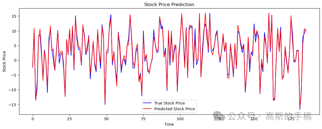
import yfinance as yfimport numpy as npimport pandas as pdfrom sklearn.preprocessing import MinMaxScalerfrom sklearn.model_selection import train_test_splitfrom sklearn.metrics import mean_absolute_error, mean_squared_error, mean_absolute_percentage_errorimport tensorflow as tffrom tensorflow.keras.models import Sequentialfrom tensorflow.keras.layers import Conv2D, MaxPooling2D, LSTM, Dense, Flatten, Dropout, BatchNormalizationimport matplotlib.pyplot as plt# Fetch stock dataticker = 'AAPL' # You can replace 'AAPL' with any ticker symboldata = yf.download(ticker, start='2020-01-01', end='2023-12-31')# Calculate additional featuresdata['SMA'] = data['Close'].rolling(window=20).mean() # Simple Moving Averagedata['EWMA'] = data['Close'].ewm(span=20, adjust=False).mean() # Exponential Moving Averagedata['Momentum'] = data['Close'] - data['Close'].shift(4) # Momentumdata['Volatility'] = data['Close'].rolling(window=20).std() # Rolling volatilitydata.dropna(inplace=True)# Use multiple features: 'Open', 'High', 'Low', 'Close', 'Volume', 'SMA', 'EWMA', 'Momentum', 'Volatility'features = data[['Open', 'High', 'Low', 'Close', 'Volume', 'SMA', 'EWMA', 'Momentum', 'Volatility']]# Normalize the datascaler = MinMaxScaler(feature_range=(0, 1))scaled_features = scaler.fit_transform(features)# Create sequencesdef create_sequences(data, seq_length):X = []y = []for i in range(len(data) - seq_length):X.append(data[i:i + seq_length])y.append(data[i + seq_length, 3]) # Using the 'Close' price as the targetreturn np.array(X), np.array(y)seq_length = 60 # Number of past days to consider for predicting the next day's priceX, y = create_sequences(scaled_features, seq_length)# Split into training and testing setsX_train, X_test, y_train, y_test = train_test_split(X, y, test_size=0.2, random_state=42)# Reshape for CNN input (Adding an extra dimension for the single channel)X_train = X_train.reshape(X_train.shape[0], X_train.shape[1], X_train.shape[2], 1)X_test = X_test.reshape(X_test.shape[0], X_test.shape[1], X_test.shape[2], 1)# Define the modelmodel = Sequential()# Adding more Conv2D layersmodel.add(Conv2D(filters=64, kernel_size=(2, X_train.shape[2]), activation='relu', input_shape=(seq_length, X_train.shape[2], 1)))model.add(BatchNormalization())model.add(MaxPooling2D(pool_size=(2, 1)))model.add(Conv2D(filters=128, kernel_size=(2, 1), activation='relu'))model.add(BatchNormalization())model.add(MaxPooling2D(pool_size=(2, 1)))model.add(Conv2D(filters=256, kernel_size=(2, 1), activation='relu'))model.add(BatchNormalization())model.add(MaxPooling2D(pool_size=(2, 1)))model.add(Flatten())# Adding more LSTM layersmodel.add(LSTM(units=100, return_sequences=True))model.add(Dropout(0.2))model.add(LSTM(units=100, return_sequences=True))model.add(Dropout(0.2))model.add(LSTM(units=50))model.add(Dropout(0.2))model.add(Dense(units=50, activation='relu'))model.add(Dense(units=1))# Compile the modelmodel.compile(optimizer='adam', loss='mean_squared_error')# Train the modelhistory = model.fit(X_train, y_train, epochs=100, batch_size=32, validation_data=(X_test, y_test))# Evaluate the modelloss = model.evaluate(X_test, y_test)print(f'Test Loss: {loss}')# Predict and inverse transform the predictionspredicted_prices = model.predict(X_test)predicted_prices = scaler.inverse_transform(np.hstack((np.zeros((predicted_prices.shape[0], 7)), predicted_prices, np.zeros((predicted_prices.shape[0], 1)))))[:, 7]# Inverse transform the true pricestrue_prices = scaler.inverse_transform(np.hstack((np.zeros((y_test.shape[0], 7)), y_test.reshape(-1, 1), np.zeros((y_test.shape[0], 1)))))[:, 7]# Calculate metricsmae = mean_absolute_error(true_prices, predicted_prices)rmse = np.sqrt(mean_squared_error(true_prices, predicted_prices))mape = mean_absolute_percentage_error(true_prices, predicted_prices)print(f'Mean Absolute Error (MAE): {mae}')print(f'Root Mean Squared Error (RMSE): {rmse}')print(f'Mean Absolute Percentage Error (MAPE): {mape}')# Calculate accuracydef calculate_accuracy(y_true, y_pred, tolerance=0.05):accurate_predictions = np.abs((y_true - y_pred) / y_true) < toleranceaccuracy = np.mean(accurate_predictions) * 100return accuracyaccuracy = calculate_accuracy(true_prices, predicted_prices)print(f'Accuracy: {accuracy:.2f}%')# Plot the resultsplt.figure(figsize=(14, 5))plt.plot(true_prices, color='blue', label='True Stock Price')plt.plot(predicted_prices, color='red', label='Predicted Stock Price')plt.title('Stock Price Prediction')plt.xlabel('Time')plt.ylabel('Stock Price')plt.legend()plt.show()
发布者:股市刺客,转载请注明出处:https://www.95sca.cn/archives/111149
站内所有文章皆来自网络转载或读者投稿,请勿用于商业用途。如有侵权、不妥之处,请联系站长并出示版权证明以便删除。敬请谅解!


