量化策略06—通道突破择时交易策略详解（下）

本文是量化策略解析系列的第6篇，本系列的内容为各种量化策略的思路和实现代码，系列连载见：

另外，我们还写有量化入门系列，详见：

在上一篇文章《通道突破择时交易策略详解（上）》中，我们介绍了如何进行通道择时、通道的类型以及通道择时的优缺点。本文将用一个具体的例子，介绍如何用Python实现通道择时策略。

一、获取基础数据

我们以上证指数为例，说明如何进行通道择时。

1. 导入需要的库

# 导入需要使用的库import akshare as akimport pandas as pdimport numpy as npimport pandas_ta as ta# 在matplotlib绘图中显示中文和负号import matplotlib.pyplot as pltimport matplotlib as mplmpl.rcParams['font.family'] = 'STKAITI' # 中文字体'STKAITI'plt.rcParams['axes.unicode_minus'] = False   # 解决坐标轴负数的负号显示问题# 关闭警告信息import warningswarnings.filterwarnings('ignore')

2. 从AKShare数据源获取上证指数的数据

关于AKShare的使用，可以参看后附的文章《如何用AKShare获取金融数据》。AKShare的接口有时会有变动，如果获取数据出错请参考AKShare的官网解决。

# 获取上证指数数据index_code = 'sh000001'start_date = pd.to_datetime('2014-01-01')end_date = pd.to_datetime('2023-12-31')price_df = ak.stock_zh_index_daily(symbol=index_code)price_df['date'] = pd.to_datetime(price_df['date']).dt.dateprice_df = price_df[(price_df['date']>=start_date) & (price_df['date']<=end_date)]price_df = price_df.sort_values('date').set_index('date')

上述代码从AKShare的stock_zh_index_daily接口获取上证指数的行情数据保存到一个名为”price_df”的DataFrame中，并选取’2014-01-01’至’2023-12-31’这10年的数据作为本例的样本数据。

3. 计算每日的收益率

# 计算每日的收益率price_df['returns'] = price_df['close'].pct_change().shift(-1).fillna(0)

上述代码用pct_change()函数计算每日的收益率。

二、计算通道

在上一篇文章中，我们介绍了5种常见的通道类型：布林带、肯特纳通道、唐奇安通道、霍尔特-温特通道和加速带。利用pandas_ta库，我们很容易就能计算这些通道的上轨、下轨和中轨。关于pandas_ta库的使用可以参看后附的文章《量化宝藏工具箱：技术指标库 Pandas TA 教程》。

下面我们分别介绍如何计算这些通道：

1. 计算布林带（Bollinger Bands）

我们可以使用pandas_ta库的bbands()函数计算布林带。

# 计算布林带（Bollinger Bands）length = 20  # 均线的周期std = 2.0  # 通道的宽度设定为几倍标准差mamode = 'sma'  # 均线的计算方式
channel = ta.bbands(price_df['close'], length=length, std=std, mamode=mamode)

bbands()函数的主要参数解析：

price_df[‘close’]：为收盘价时间序列；

length：为计算均线的周期，本例中取值20，表示计算20日均线；

std：为通道宽度，本例取值2.0，表示通道的上轨和下轨距离中轨都是2个标准差；

mamode：为均线的计算方式，本例中’sma’表示用简单移动平均线来计算中轨。pandas_ta库支持多种均线，详情可以常见后附的文章《
均线解密：如何有效利用移动平均线》。

布林带的计算结果如下：

表中的各列为：BBL、BBM、BBU分别为布林带的下轨、中轨和上轨；BBB为通道的宽度；BBP为价格在布林带中的位置。列名的后缀”_20_2.0″为布林带函数的参数length和std的值。

2. 计算肯特纳通道（Keltner Channels）

可以用pandas_ta库的kc()函数来计算肯特纳通道。

# 计算肯特纳通道（Keltner Channels）length = 20  # 均线的周期scalar = 2  # 通道的宽度设定为几倍ATRmamode = 'ema'  # 均线的计算方式
channel = ta.kc(price_df['high'], price_df['low'], price_df['close'], length=length, scalar=scalar, mamode=mamode)

kc()函数的主要参数解析：

price_df[‘high’], price_df[‘low’], price_df[‘close’]：分别为最高价、最低价、收盘价的时间序列；

length：为计算均线的周期，本例中取值20，表示计算20日均线；

scalar：为通道宽度，本例取值2.0，表示通道的上轨和下轨距离中轨都是2倍的ATR；

mamode：为均线的计算方式，本例中’ema’表示用简单移动平均线来计算中轨。

肯特纳通道的计算结果如下：

表中的KCLe、KCBe、KCUe分别为肯特纳通道的下轨、中轨和上轨。列名的后缀”_20_2.0″为肯特纳通道函数的参数length和scalar的值。

3. 计算唐奇安通道（Donchian Channels）

可以用pandas_ta库的donchian()函数计算唐奇安通道。

# 计算唐奇安通道（Donchian Channels）length = 20  # 最高价、最低价的周期channel = ta.donchian(price_df['high'], price_df['low'], lower_length=length, upper_length=length)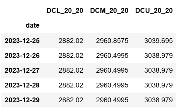

donchian()函数的主要参数解析：

price_df[‘high’], price_df[‘low’]：最高价和最低价的时间序列；

lower_length：计算下轨时用到的周期数，本例中为20日；

upper_length：计算上轨时用到的周期数，本例中为20日。

唐奇安通道的计算结果如下：

表中的DCL、DCM、DCU分别为唐奇安通道的下轨、中轨和上轨。列名的后缀”_20_20″为唐奇安通道函数的参数lower_length和upper_length的值。

4. 计算霍尔特-温特通道（Holt-Winter Channel）

可以用pandas_ta库的hwc()函数计算霍尔特-温特通道。

# 计算霍尔特-温特通道（Holt-Winter Channel）channel = ta.hwc(price_df['close'])

hwc()函数的主要参数price_df[‘close’]为收盘价的时间序列。

霍尔特-温特通道的计算结果如下：

表中的HWM、HWU和HWL分别为霍尔特-温特通道的中轨、上轨和下轨。

5. 计算加速带（Acceleration Bands）

可以用pandas_ta库的accbands()函数计算加速带。

# 计算加速带（Acceleration Bands）length = 20  # 均线的周期mamode = 'sma'  # 均线的计算方式
channel = ta.accbands(price_df['high'], price_df['low'], price_df['close'], length=length, mamode=mamode)

accbands()函数的主要参数解析：

price_df[‘high’], price_df[‘low’], price_df[‘close’]：为最高价、最低价和收盘价的时间序列；

length：为计算均线的周期，本例中取值20，表示计算20日均线；

mamode：为均线的计算方式，本例中’sma’表示用简单移动平均线来计算中轨。

加速带的计算结果如下：

表中的ACCBL、ACCBM、ACCBU列分别为加速带的下轨、中轨和上轨。列名的后缀”_20″为加速带函数的参数length的值。

6. 可视化输出通道图形

以布林带为例，可视化输出通道图形：

# 可视化输出通道# 通道上轨、下轨、中轨的名称up = 'BBU_20_2.0'down = 'BBL_20_2.0'middle = 'BBM_20_2.0'
channel[[up, down, middle]].plot(figsize=(10, 6))

结果为：

三、构建通道突破择时策略

我们以布林带为例，构建通道突破择时策略如下：

1. 计算择时信号

本例采用趋势交易策略，择时信号为：价格突破通道上轨时开仓，价格跌破通道下轨时清仓，价格在通道内时维持先前的仓位。

# 计算择时信号:价格突破通道上轨时开仓,价格跌破通道下轨时清仓,价格在通道内时维持先前的仓位timing_df = pd.DataFrame()timing_df['择时'] = (price_df['close']>=channel[up]) * 1. + (price_df['close']<=channel[down]) * -1.timing_df = timing_df.replace(0, np.nan)  # 先将0替换为NAtiming_df = timing_df.fillna(method='ffill').fillna(0)  # 使用前值填充NAtiming_df[timing_df<0] = 0timing_df['不择时'] = 1.

上述代码的作用是基于给定的价格数据和通道数据来创建一个包含择时信号的DataFrame表。timing_df表的’择时’列用于记录择时信号，其中高于上轨的位置被视为买入信号（1.0）；而低于下轨的位置原本被视为卖出信号（最开始值为-1.0，后来被调整为0）；通道中的位置最开始的值为0，后来调整为与前一个非0值一致。表中还包括一个一直持有的信号列（’不择时’），表示不进行择时操作的策略。

2. 计算择时效果

# 计算择时和不择时的每日收益率timing_ret = timing_df.mul(price_df['returns'], axis=0)timing_ret['超额收益'] = (1+timing_ret['择时']).div(1+timing_ret['不择时'], axis=0) - 1.# 计算累计收益率cumul_ret = (1 + timing_ret.fillna(0)).cumprod() - 1.

这段代码用来用以计算和比较择时策略与不择时策略的收益表现。首先将timing_df中的择时信号与price_df中的每日收益率相乘。择时信号为1时（表示择时策略持有资产），将直接取该资产的日收益率；为0时（表示择时策略未持有资产），收益率为0。然后，根据择时的日收益和不择时的日收益计算择时带来的超额收益。最后，通过日收益率的累积乘积计算累计的收益率。

关于各种收益的计算，可以参看后附的文章《一文讲清7种收益率的python实现》和《计算超额收益，你用减法还是除法》。

3. 将择时效果可视化输出

# 可视化输出cumul_ret.plot(figsize=(10, 6), title='通道择时')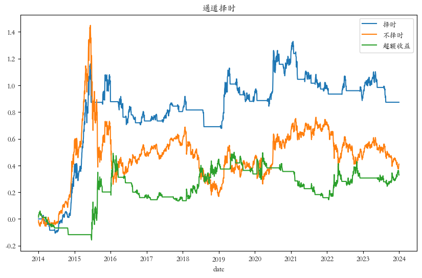

结果如下：

从上图可以看到，利用布林带择时的收益要高于不择时的收益。同时，从超额收益曲线也可以看出择时的超额收益并不稳定。当然，本例只是说明通道择时如何实现，并未对择时方案进行优化。大家可以对择时方案进行调整，例如选取其他通道类型，或修改通道的参数，以达到更好的择时效果。

通道突破择时交易策略详解（上）

量化宝藏工具箱：技术指标库 Pandas TA 教程

发布者：股市刺客，转载请注明出处：https://www.95sca.cn/archives/106000
站内所有文章皆来自网络转载或读者投稿，请勿用于商业用途。如有侵权、不妥之处，请联系站长并出示版权证明以便删除。敬请谅解！

量化策略06—通道突破择时交易策略详解（下）

相关推荐

发表回复