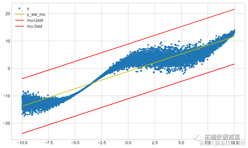
这在模型噪声随着模型变量之一变化或为非线性的情况下特别有用，比如在存在异方差性的情况下。

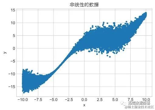
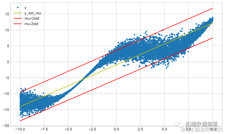
当客户的数据是非线性时，这样会对线性回归解决方案提出一些问题：

# 添加的噪声量是 x 的函数
n = 20000

......
x_train = x[: n // 2]
x_test = x[n // 2 :]
y_train = y[: n // 2]
......
plt.show()

线性回归方法

我们用均方差作为优化目标，这是线性回归的标准损失函数。

model_lin_reg = tf.keras.Sequential(
......
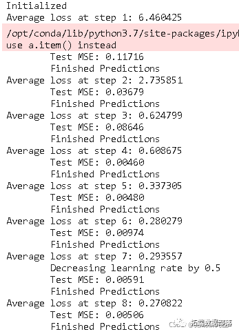
history = model_lin_reg.fit(x_train, y_train, epochs=10, verbose=0)
# 模型已经收敛：
plt.plot(history.history["loss"])
......

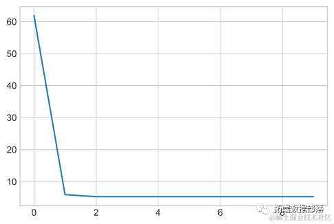
Final loss: 5.25

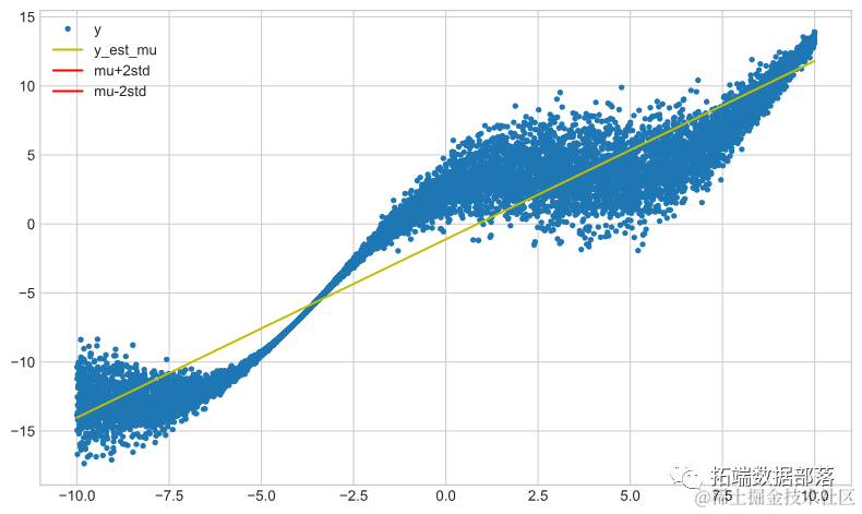
我们定义一些辅助函数来绘制结果：

def plot_results(x, y, y_est_mu, y_est_std=None):
  ......
    plt.show()


def plot_model_results(model, x, y, tfp_model: bool = True):
    model.weights

......
    plot_results(x, y, y_est_mu, y_est_std)

模型残差的标准差不影响收敛的回归系数，因此没有绘制。

plot_modesults(mod_linreg......, tfp_model=False)

---

01

02

03

04

TensorFlow概率

我们可以通过最大化正态分布的似然性来拟合上述相同的模型，其中平均值是线性回归模型的估计值。

def negloglik(y, distr):
  ......


model_lin_reg_tfp = tf.keras.Sequential(
 ......
            lambda t: tfp.distributions.Normal(loc=t, scale=5,)
        ),
    ]
)

model_lin_reg_tfp.compile(
......)

history = model_lin_reg_tf......
plot_model_results(model_lin_r......rue)

拟合带有标准差的线性回归

为了拟合线性回归模型的最佳标准差，我们需要进行一些操作。我们需要网络输出两个节点，一个用于表示平均值，另一个用于表示标准差。

model_lin_reg_std_tfp = tf.keras.Sequential(
    [
  ......
        ),
    ]
)

model_lin_reg_std_tfp.compile(
......)

history = model_lin_reg_std_tfp.fit(x_train, y_train, epochs=50, ......train, tfp_model=True)

上面的图表显示，标准差和均值都与之前不同。它们都随着x变量的增加而增加。然而，它们对数据仍然不是很好的拟合，无法捕捉到非线性关系。

神经网络方法

为了帮助拟合x和y之间非线性关系，我们可以利用神经网络。这可以简单地使用我们设计的相同TensorFlow模型，但添加一个具有非线性激活函数的隐藏层。

model_lin_reg_std_nn_tfp = tf.keras.Sequential(
    [
 ......
            )
        ),
    ]
)

model_lin_reg_std_nn_tfp.compile(
   ......
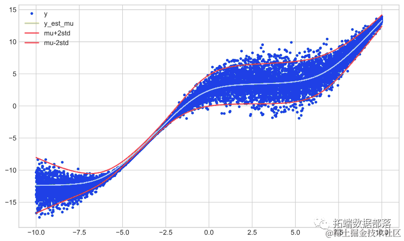
plot_model_results(mode ......rain, tfp_model=True)

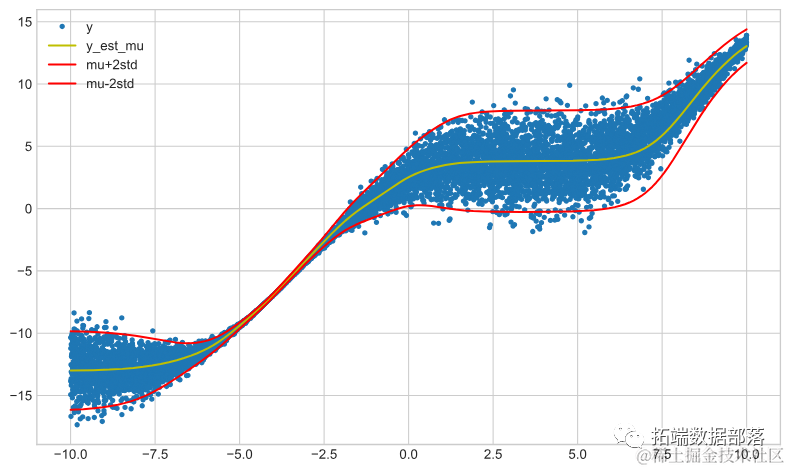
神经网络模型拟合的均值比线性回归模型更好地符合数据的非线性关系。

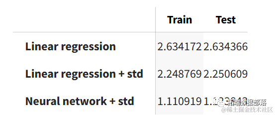
结果

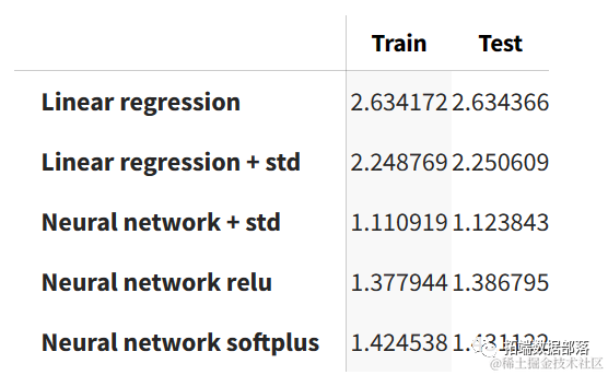
我们对训练集和测试集运行了各个模型。在任何模型中，两者之间的性能变化不大。我们可以看到，神经网络模型在训练集和测试集上的表现最好。

results = pd.DataFrame(index=["Train", "Test"])

models = {
  ......
        ).numpy(),
    ]
results.transpose()

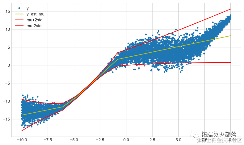
激活函数

下面使用relu或softplus激活函数创建相同的网络。首先是relu网络的结果：

model_relu = tf.keras.Sequential(
    [
  ......
                loc=t[:, 0:1], scale=tf.math.softplus(t[:, 1:2])
            )
        ),
    ]
)

m ......
plot_model_results(model_relu, x_train, y_train)

然后是softplus的结果：

model_softplus = tf.keras.Sequential(
    [
  ......
                loc=t[:, 0:1], scale=tf.math.softplus(t[:, 1:2])
            )
        ),
    ]
)

model_softplus.compile(
 ......
plot_model_results(model_softplus, x_train, y_train)

 我们可以看到，基于sigmoid的神经网络具有最佳性能。

results = pd.DataFrame(index=["Train", "Test"])

models = {
 ......(x_test))
        ).numpy(),
    ]
results.transpose()