
在上一篇文章《择时新思路:波动率与换手率中的牛熊密码(上)》中,我们介绍了用波动率和换手率构建牛熊指标进行择时的思路。本文将用一个具体的例子说明如何用Python实现牛熊指标择时。
# 导入需要使用的库import akshare as akimport pandas as pdimport numpy as npimport pandas_ta as ta# 在matplotlib绘图中显示中文和负号import matplotlib.pyplot as pltimport matplotlib as mplmpl.rcParams['font.family'] = 'STKAITI' # 中文字体'STKAITI'plt.rcParams['axes.unicode_minus'] = False # 解决坐标轴负数的负号显示问题# 关闭警告信息import warningswarnings.filterwarnings('ignore')# 获取指数数据index_code = '000300'start_date = pd.to_datetime('2010-01-01')end_date = pd.to_datetime('2023-12-31')price_df = ak.index_zh_a_hist(symbol=index_code, period="daily", start_date=start_date, end_date=end_date)price_df['日期'] = pd.to_datetime(price_df['日期'])price_df = price_df.sort_values('日期').set_index('日期')

# 计算每日的涨跌幅(即日收益率)price_df['涨跌幅'] = price_df['收盘'].pct_change().fillna(0)# 将日收益率向上位移1位,用于计算策略收益,避免涉及未来数据price_df['returns'] = price_df['涨跌幅'].shift(-1)牛熊指标 = 波动率 / 换手率其中:波动率:为某个时间段内股票指数日收益率的标准差换手率:为同一时间段内股票指数日换手率的移动平均值# 计算滚动窗口的波动率days = 244price_df[f'波动率_{days}'] = price_df['涨跌幅'].rolling(days, min_periods=int(days/2)).std()# 计算移动平均的换手率price_df[f'换手率_{days}'] = price_df['换手率'].rolling(days, min_periods=int(days/2)).mean()# 计算牛熊指标price_df['牛熊指标'] = price_df[f'波动率_{days}'] / price_df[f'换手率_{days}']# 可视化指数与牛熊指标的关系fig, ax1 = plt.subplots(figsize = (10,6))# 指数收盘价曲线ax1.plot(price_df['收盘'], label='收盘价', color='r')plt.legend(loc='upper left')# 牛熊指标曲线ax2 = ax1.twinx() ax2.plot(price_df['牛熊指标'], label='牛熊指标', color='b')ax2.legend(loc = 'best')ax1.set_title(f'指数{index_code}收盘价与牛熊指标')plt.show()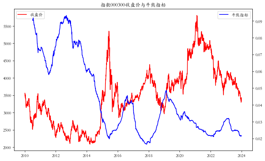
# 计算指数与牛熊指标的相关系数corr = price_df['收盘'].corr(price_df['牛熊指标'])print(f'指数{index_code}与牛熊指标的相关系数为:',corr)# 计算牛熊指标的双均线days_s = 20 # 短均线天数days_l = 60 # 长均线天数price_df[f'牛熊指标_ma{days_s}'] = ta.sma(price_df['牛熊指标'], length=days_s)price_df[f'牛熊指标_ma{days_l}'] = ta.sma(price_df['牛熊指标'], length=days_l)# 根据牛熊指标的长短均线计算择时信号timing_df = pd.DataFrame()timing_df['牛熊指标择时'] = ~(price_df[f'牛熊指标_ma{days_s}']>price_df[f'牛熊指标_ma{days_l}']) * 1.# 计算指数的双均线price_df[f'指数_ma{days_s}'] = ta.sma(price_df['收盘'], length=days_s)price_df[f'指数_ma{days_l}'] = ta.sma(price_df['收盘'], length=days_l)# 计算择时信号:当指数的短均线在长均线之上时开仓,反之清仓timing_df['指数均线择时'] = (price_df[f'指数_ma{days_s}']>price_df[f'指数_ma{days_l}']) * 1.timing_df['不择时'] = 1.# 计算择时和不择时的每日收益率timing_ret = timing_df.mul(price_df['returns'], axis=0)
# 计算累计收益率cumul_ret = (1 + timing_ret.fillna(0)).cumprod() - 1.# 可视化择时效果cumul_ret.plot(figsize = (10,6))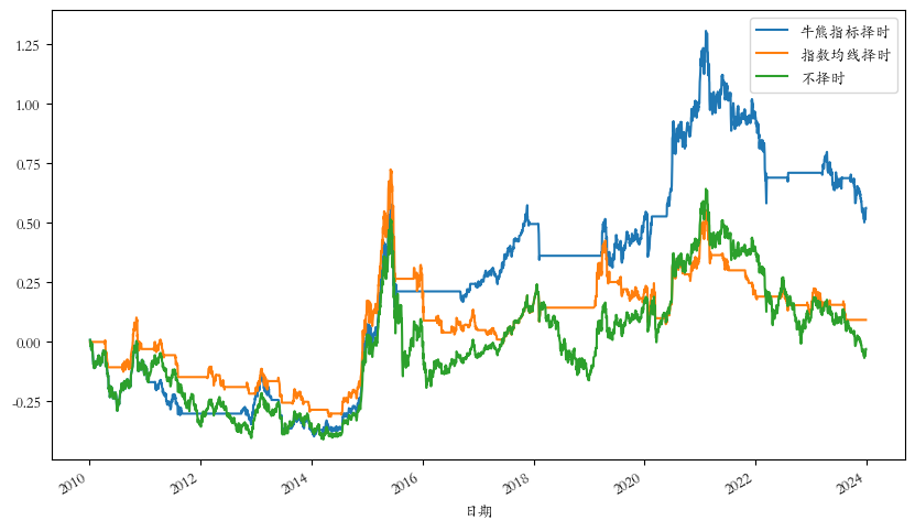
发布者:股市刺客,转载请注明出处:https://www.95sca.cn/archives/105995
站内所有文章皆来自网络转载或读者投稿,请勿用于商业用途。如有侵权、不妥之处,请联系站长并出示版权证明以便删除。敬请谅解!